Mapping Global Land Cover with European Space Agency Data
Introduction: The ESA WorldCover dataset
The European Space Agency's WorldCover is a freely accessible dataset providing global land cover classification at 10-meter resolution derived from Sentinel-1 and Sentinel-2 satellite imagery. Released in 2020 and updated in 2021, the ESA reports that the updated dataset achieves an overall accuracy of 76.7% in identifying land cover types, including forests, grasslands, croplands, urban areas, and water bodies across the entire Earth's surface.
The high-resolution imagery WorldCover offers is especially valuable for environmental monitoring, urban planning, and understanding how human activity impacts and encroaches upon wild landscapes. WorldCover's 10-meter resolution can capture fine-grained details such as the difference a small forest patch and an adjacent agricultural field, or between building clusters within a neighborhood. The ESA distributes WorldCover imagery through several access points, including through two WMTS services (one for the 2020 product, and another for the 2021 version). You can find a list of these access points at this link.
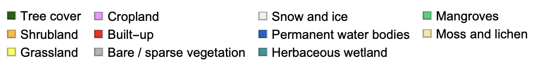
ESA WorldCover classifies land cover using the following eleven land cover classes:
In Wolfram Language (WL), it's fairly straightforward to access ESA WorldCover data through GeoGraphics using the GeoServer option. This way, we can visualize land cover for any region on Earth, from small scale features like countryside human settlements to entire continents, and compare it to other geographic data to uncover patterns in land use and other anthropogenic environmental impacts.
This short piece will demonstrate how to connect to ESA WorldCover to make custom geographic visualisations in WL, and illustrate the flexibility of the Wolfram environment for this kind of data exploration by visualizing the land cover around the twenty largest US cities by population size, and around the 63 US national parks. The code to generate the former set of maps will be about five lines long, and about twenty lines long for the latter.
Connecting to ESA WorldCover with GeoGraphics
First, let's define the GeoServer options to access the WorldCover datasets.
GeoServer specification for ESA WorldCover 2020:
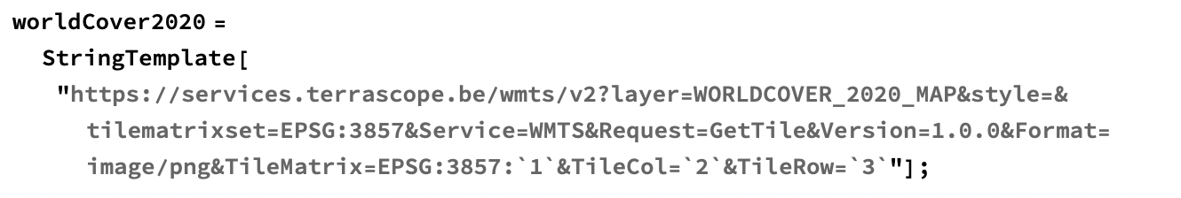
GeoServer specification for ESA WorldCover 2021:
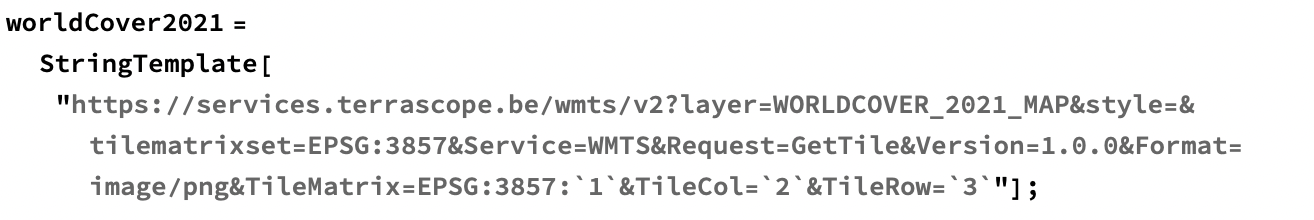
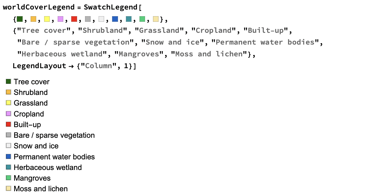
While we're at it, let's define a legend with which to label our maps.
Define a WorldCover legend:
We now have all the pieces needed to make WorldCover visualizations. To make a land cover map, simply call specify the region you'd like to plot and the GeoServer specification to use inside GeoGraphics.
Map global land cover:
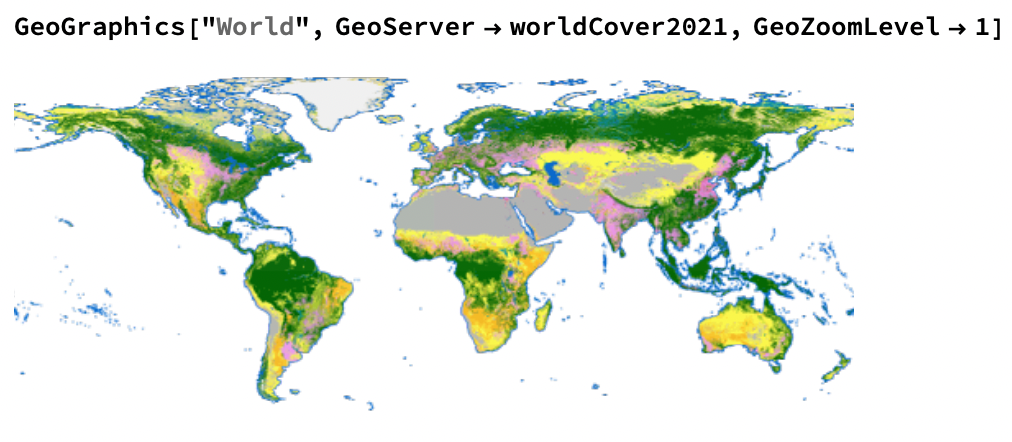
I've specified the GeoZoomLevel option manually in this example because the default setting results in imagery just below the resolution I want. This is a side-effect of the way the ESA WorldCover data services are set up. Let's come back to that later. For now, we'll keep specifying the zoom level manually.
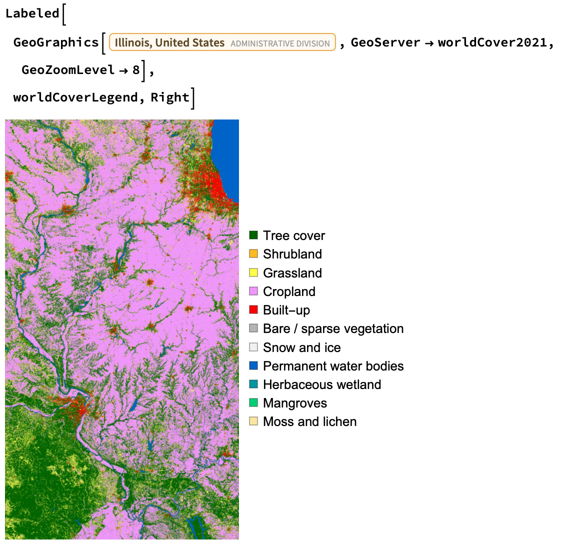
To add the legend we defined above to the plot, you can use Labeled. The main advantage of using Labeled over Legended is that you can control where the legend goes with the third argument. If the example below had resulted in a wide map, for instance, we might have instead chosen to add the legend below the map using Below as the third argument to Labeled instead of Right.
Map the land cover in Illinois:
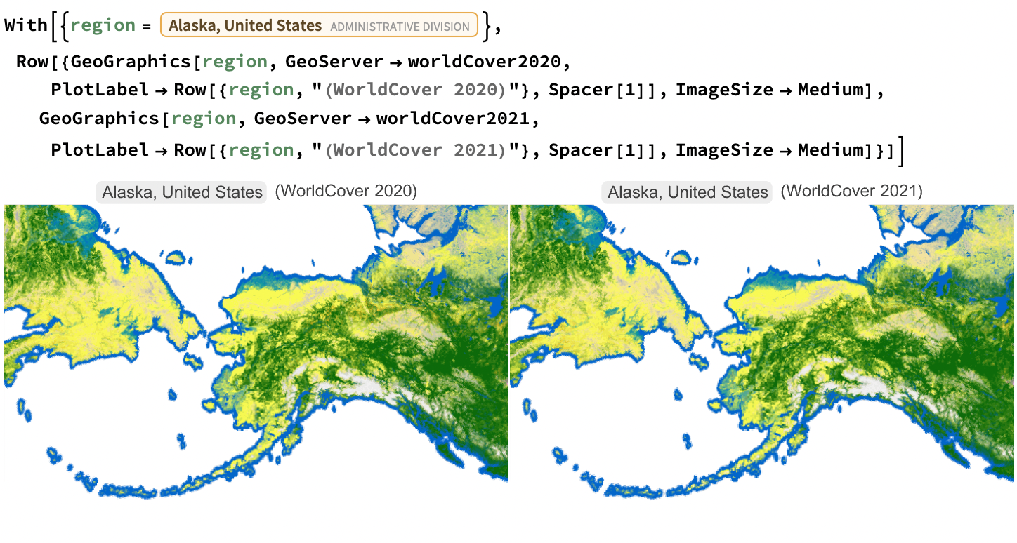
We can easily compare both dataset versions by plotting the same map twice, once with each GeoServer specification.
Compare imagery from WorldCover 2020 and WorldCover 2021 over the same region:
By lightly modifying the previous example, we can make a side-by-side comparison of ESA WorldCover land cover classification with another map of the same region:
Map the land cover around London:

Since the WorldCover dataset has global coverage, it can be used to visualise land cover for remote areas.
Map the land cover on Kerguelen:

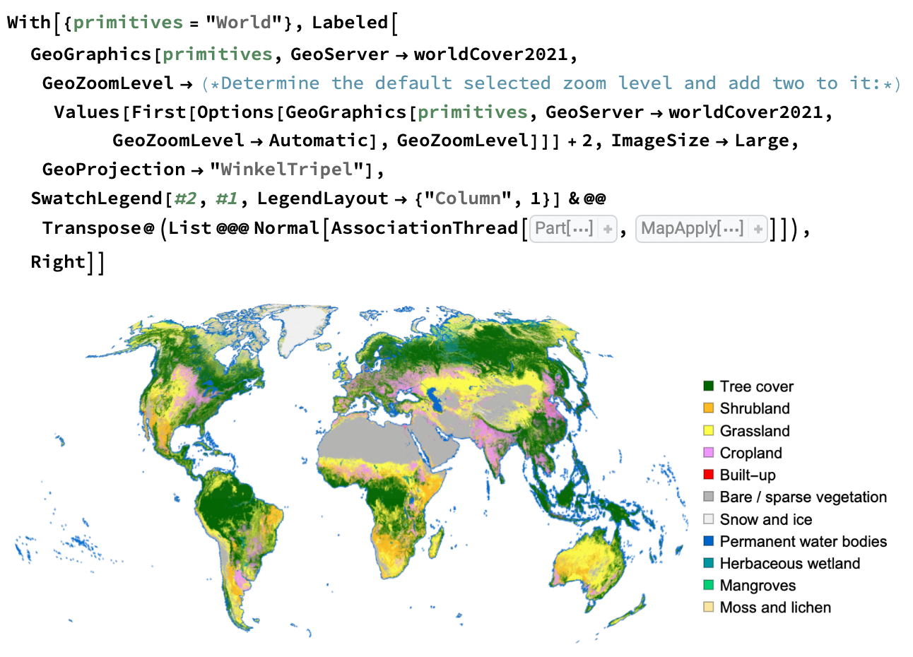
To adjust the automatic GeoZoomLevel setting I've opted to generate the map once with automatic settings, retrieving the chosen GeoZoomLevel from the result and adding a constant (I chose 2) to the result to get the adjusted setting to use in the final map. Then I recompute the final map with the adjusted GeoZoomLevel.
Automatically set the zoom level to be a little higher than by default:
In the following sections, I'll apply the connection to this dataset to automatically survey the land cover around the largest US cities by population, and all 63 US national parks.
Land cover around major US cities
We can apply this workflow to quickly visualize any set of locations. Let's start with the largest cities in the US.
List the largest US cities by population:

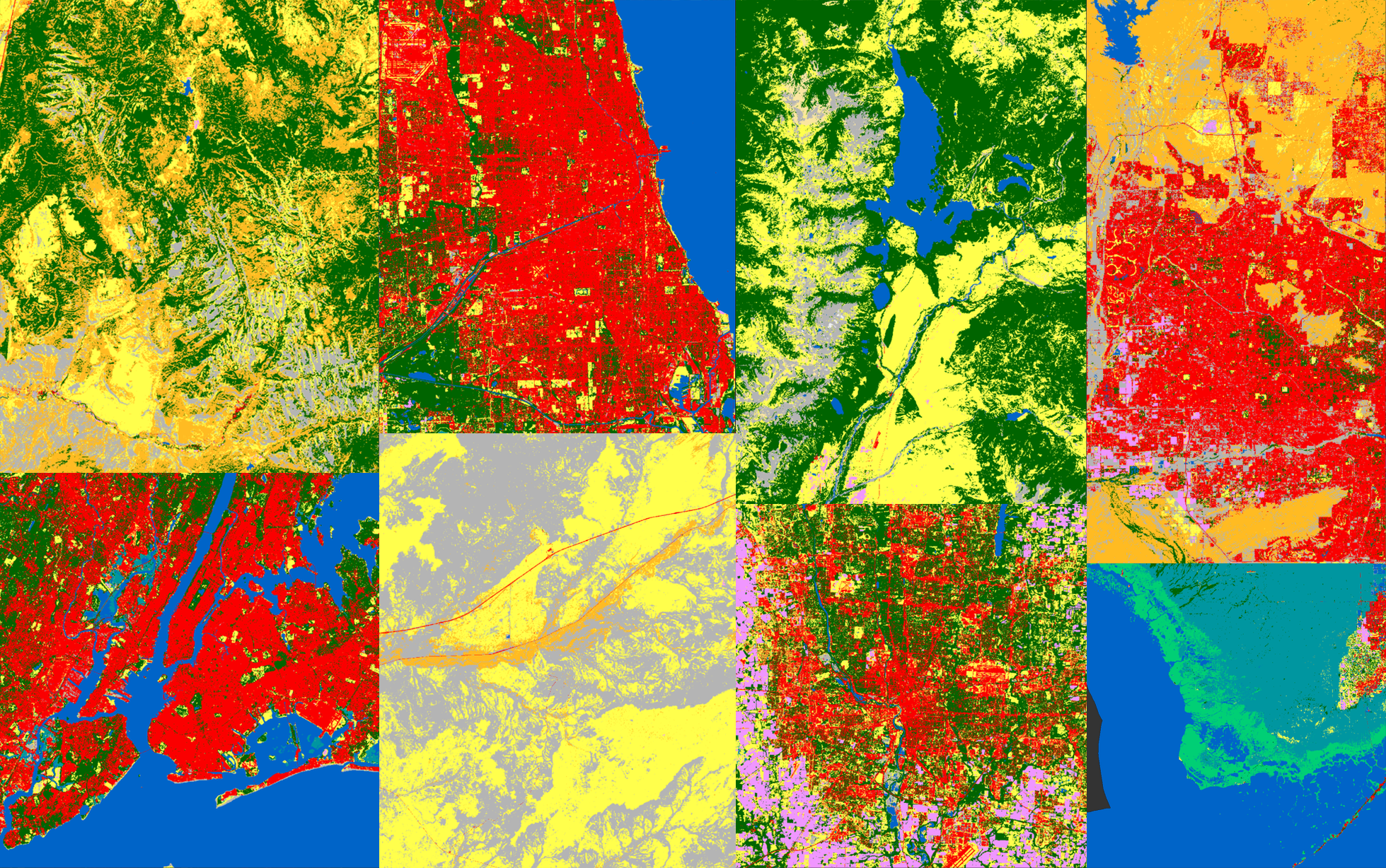
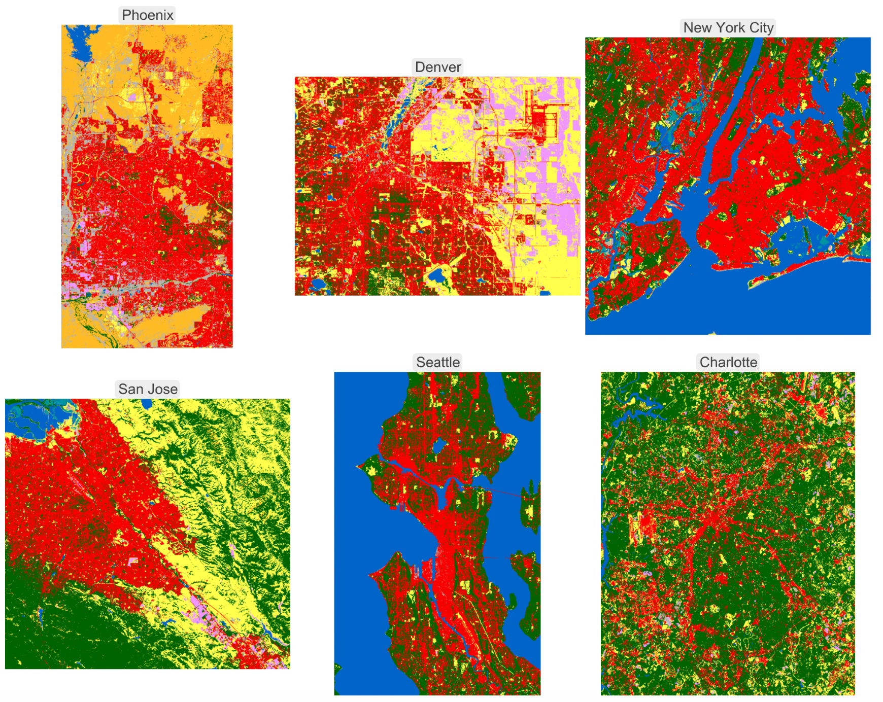
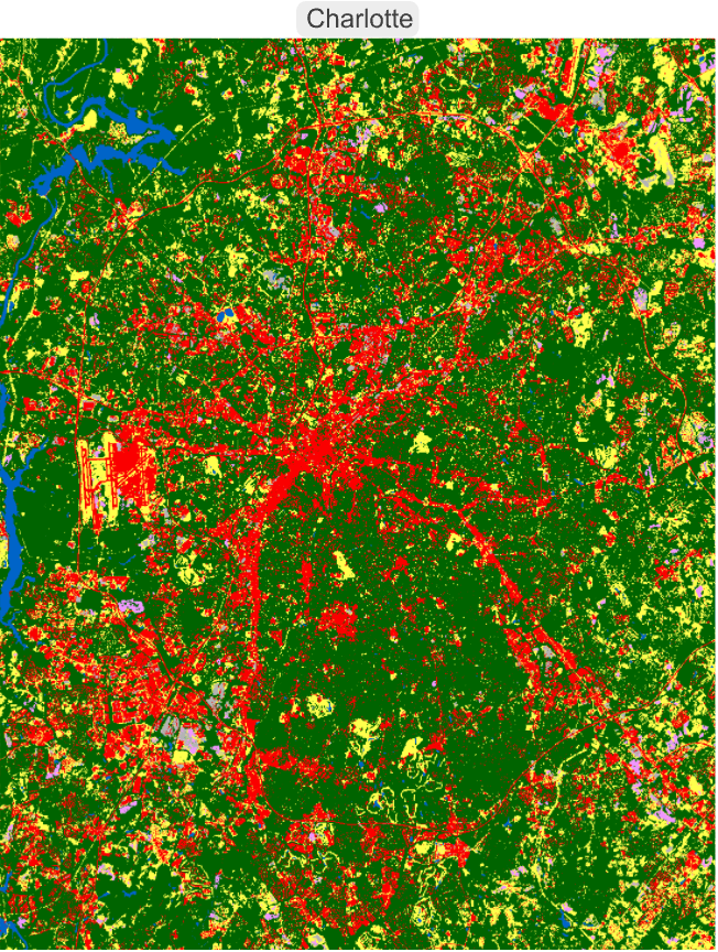
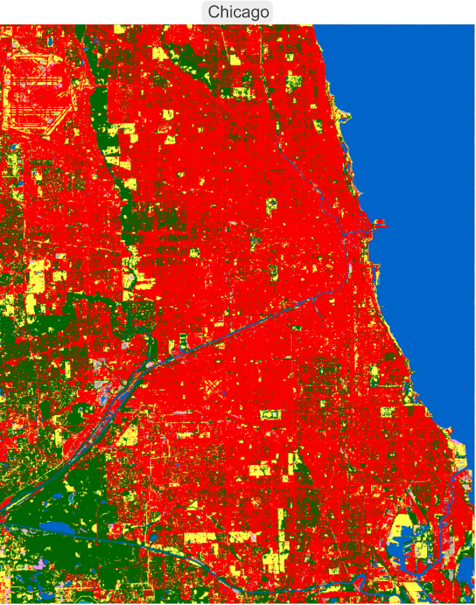
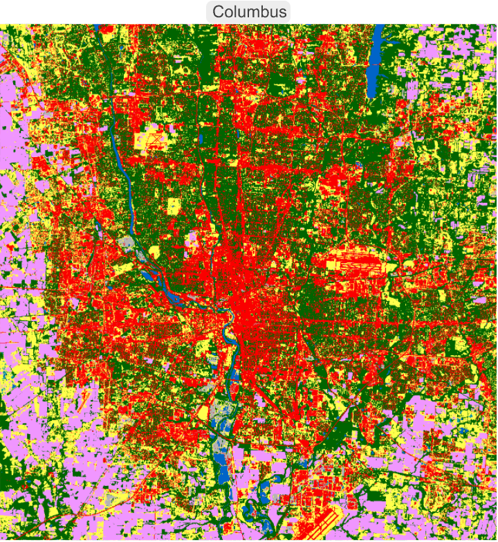
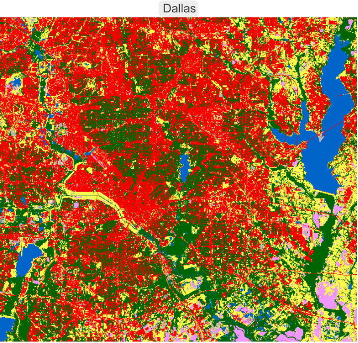
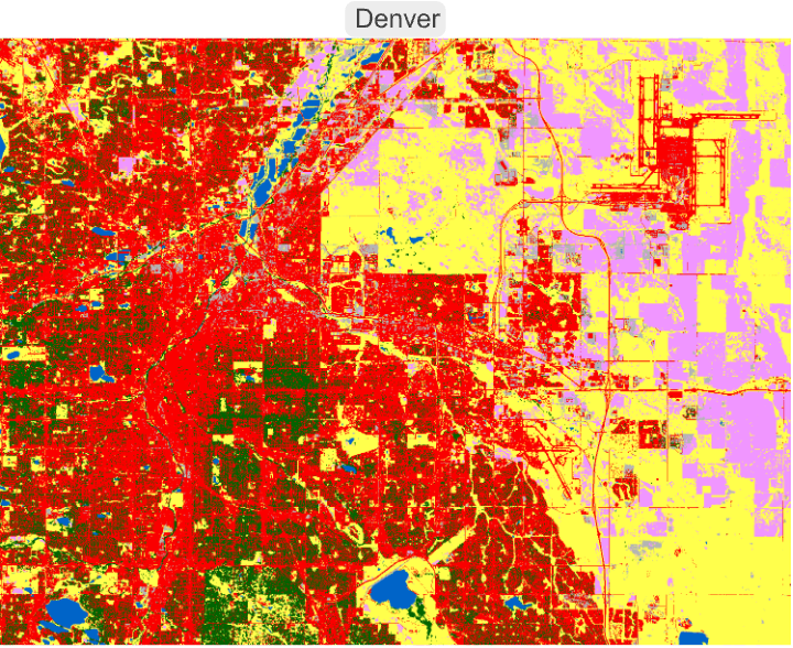
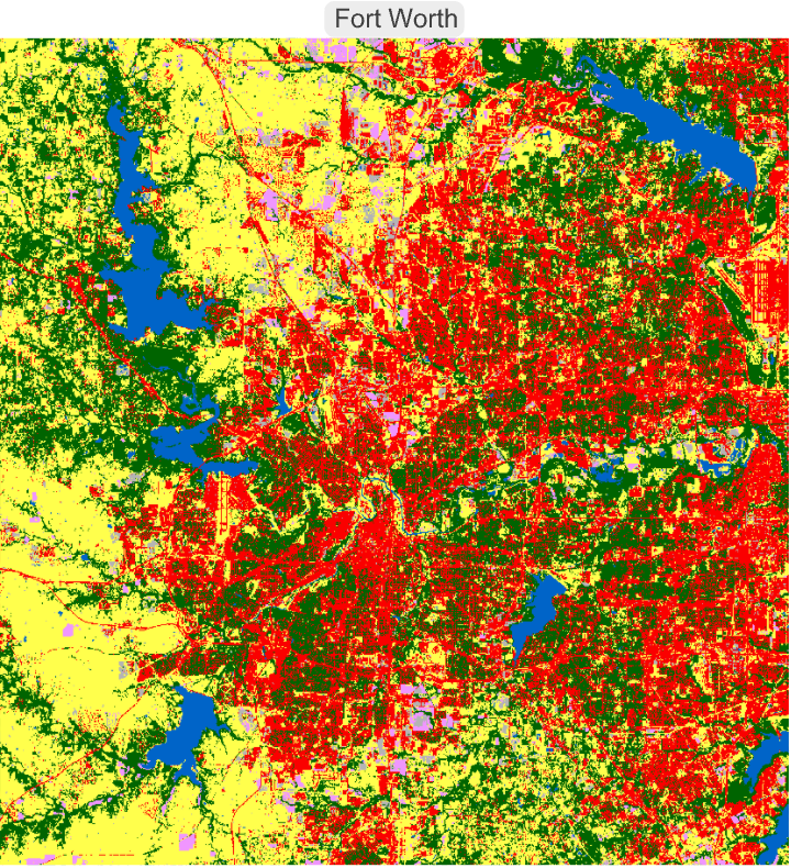
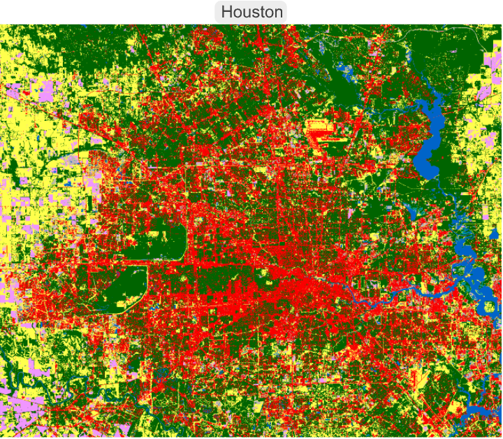
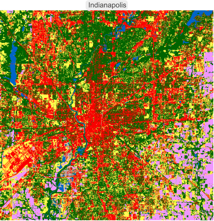
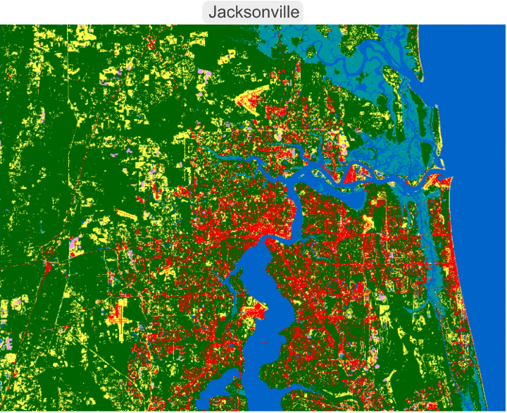
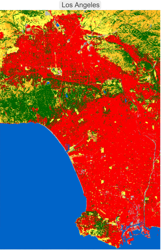
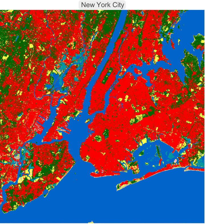
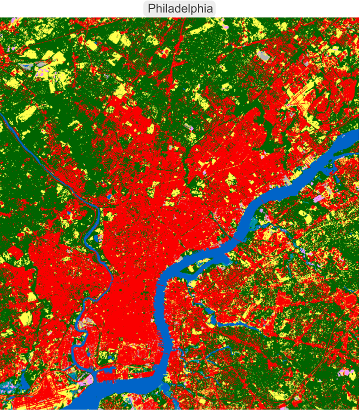
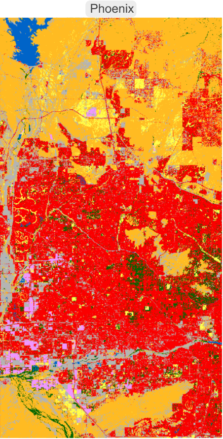
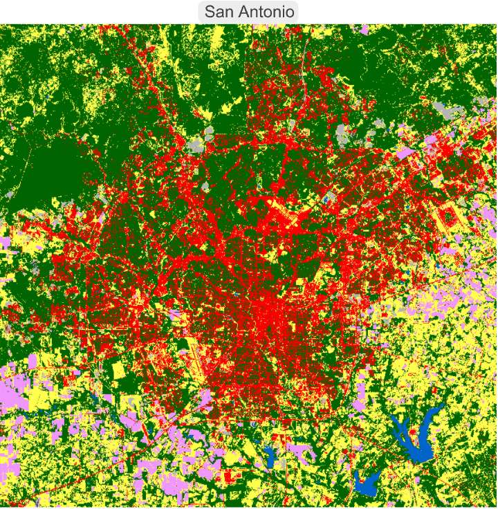
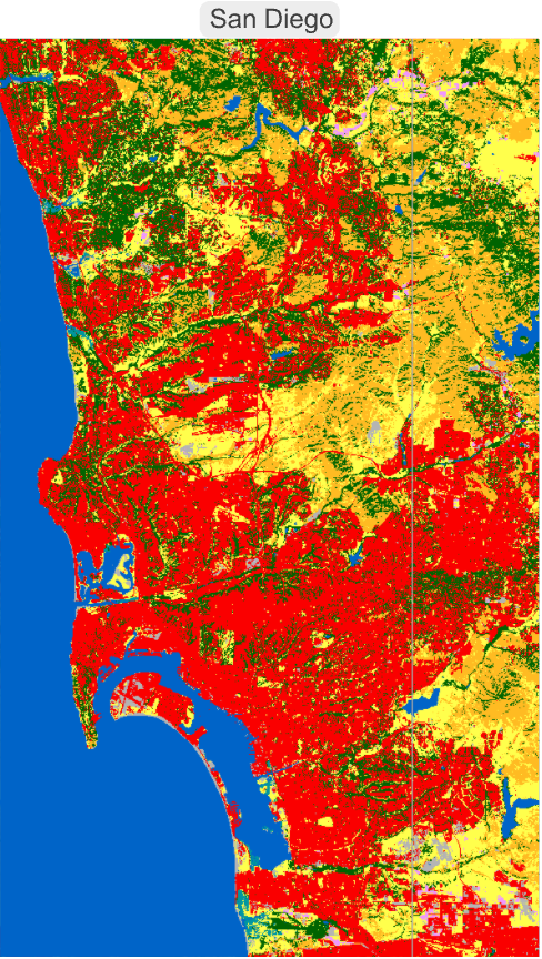
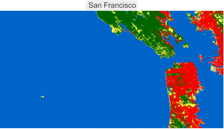
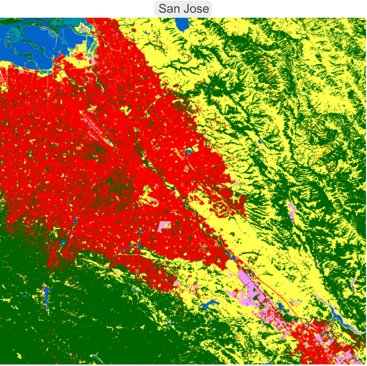
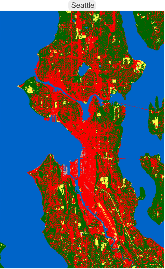
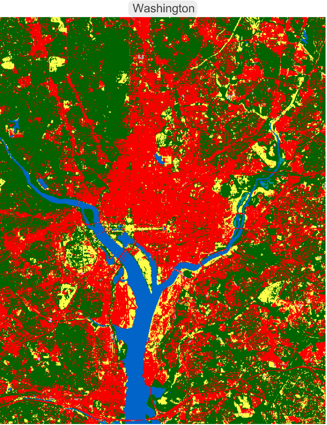
Plotting the ESA land cover for these cities yields important morphological visual contrasts. For example, Phoenix and Denver exemplify contiguous expansion into open terrain and are surrounded by arid shrubland and high plains grassland, respectively. In contrast, New York, San Jose and Seattle have sharp boundaries where development is strictly confined by valley topography or water bodies, and in Charlotte the built environment is heavily interspersed with dense tree canopy.
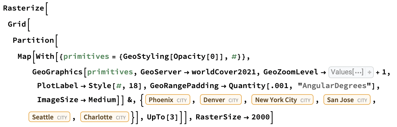
Map the land cover around any of the twenty largest US cities by population:
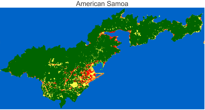
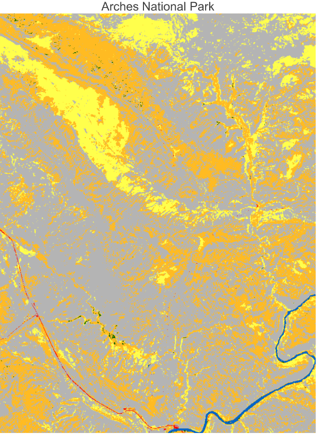
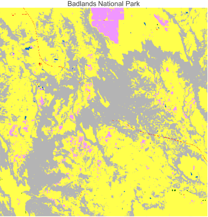
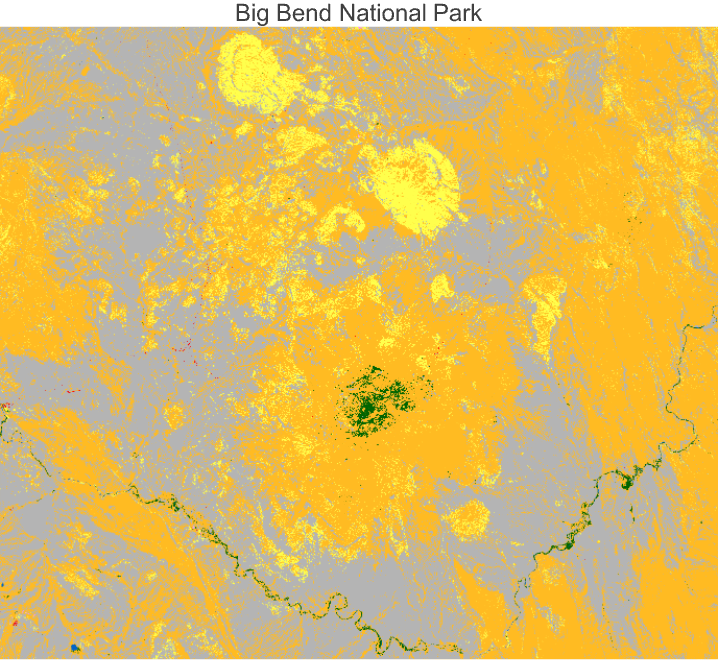
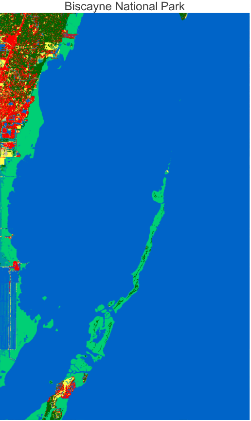
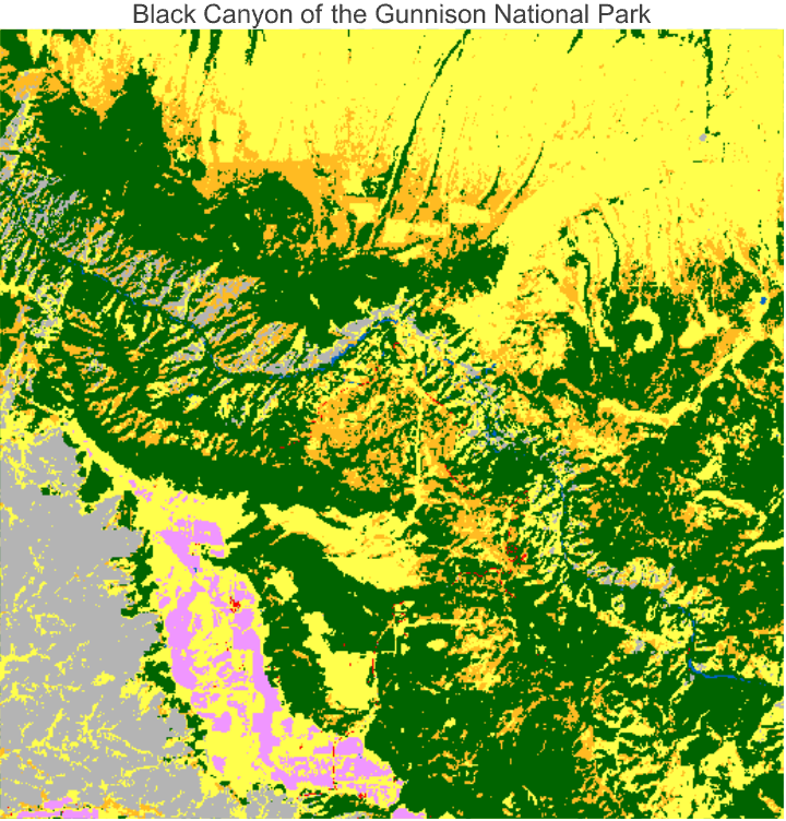
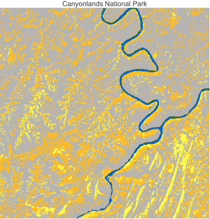
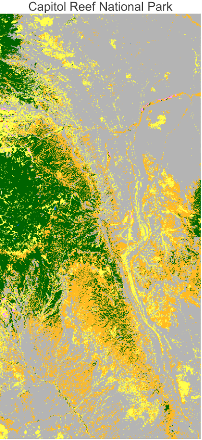
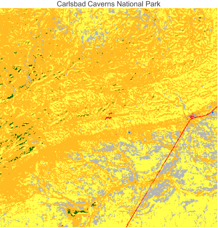
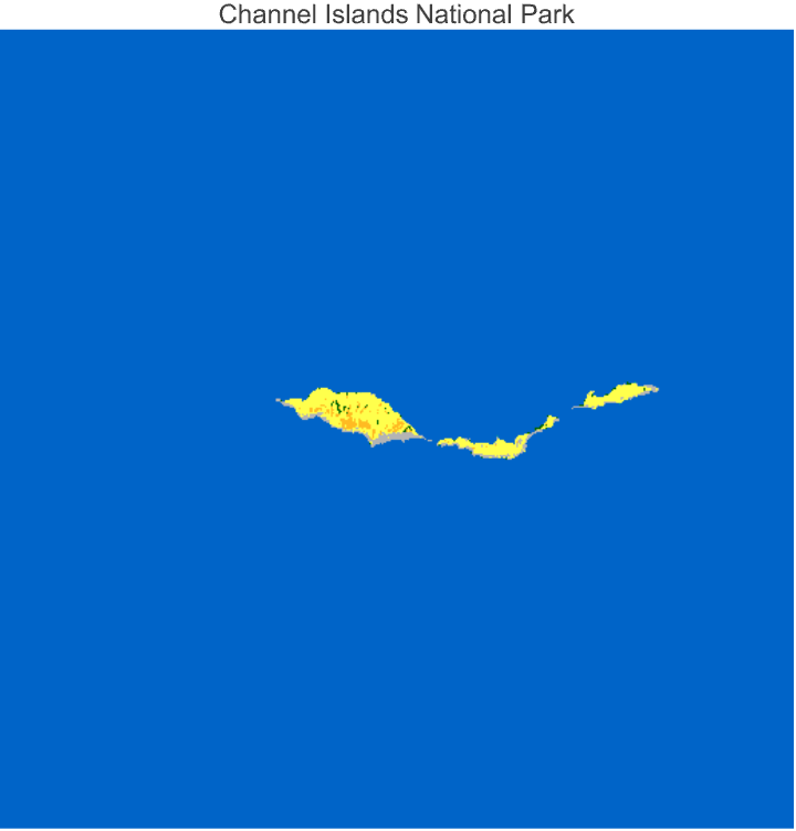
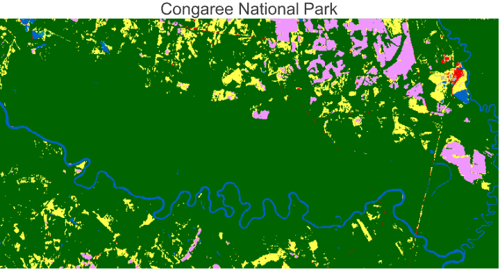
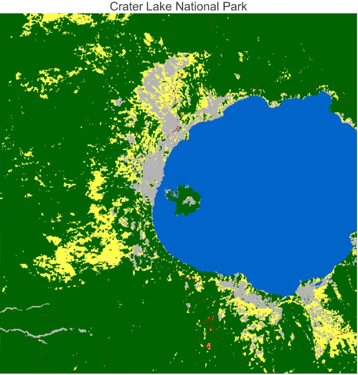
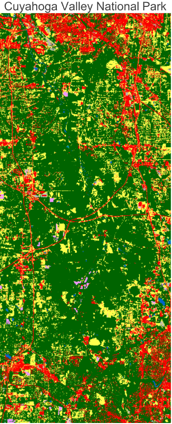
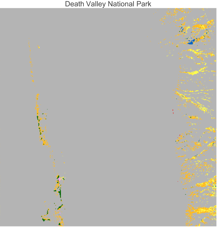
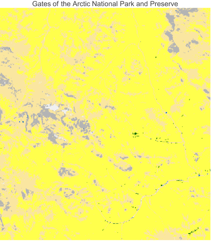
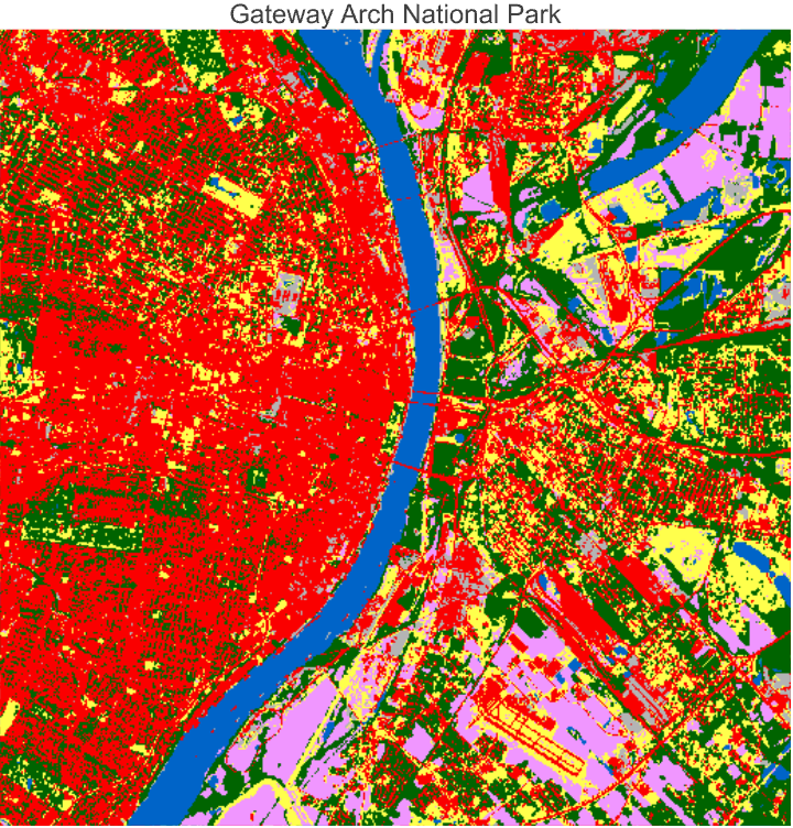
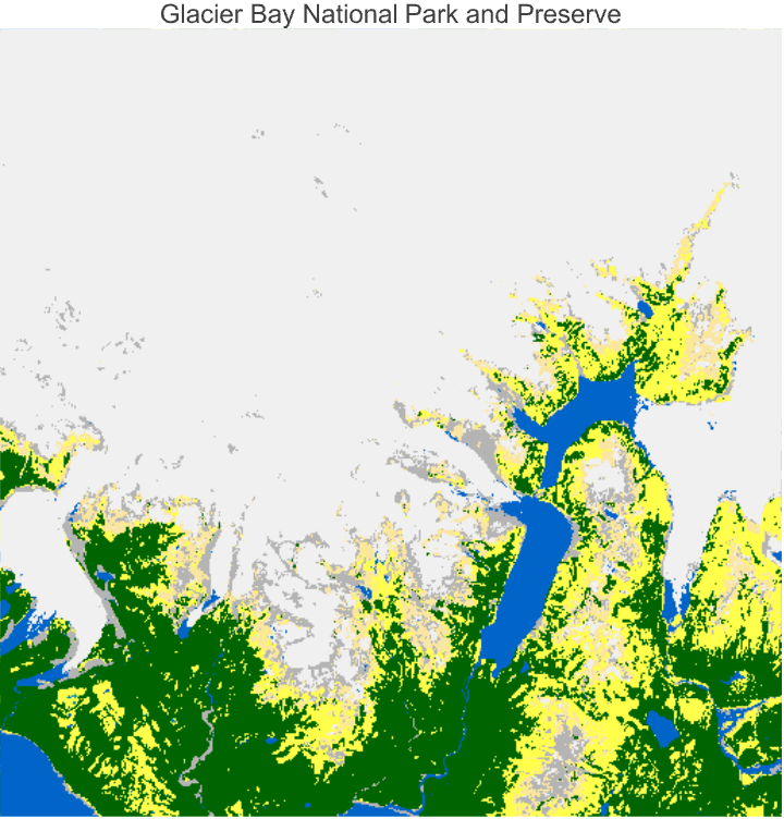
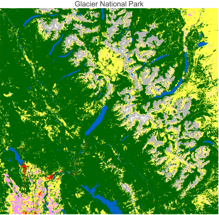
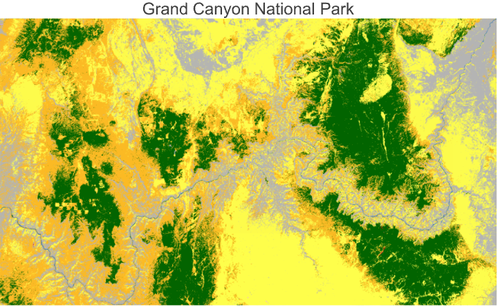
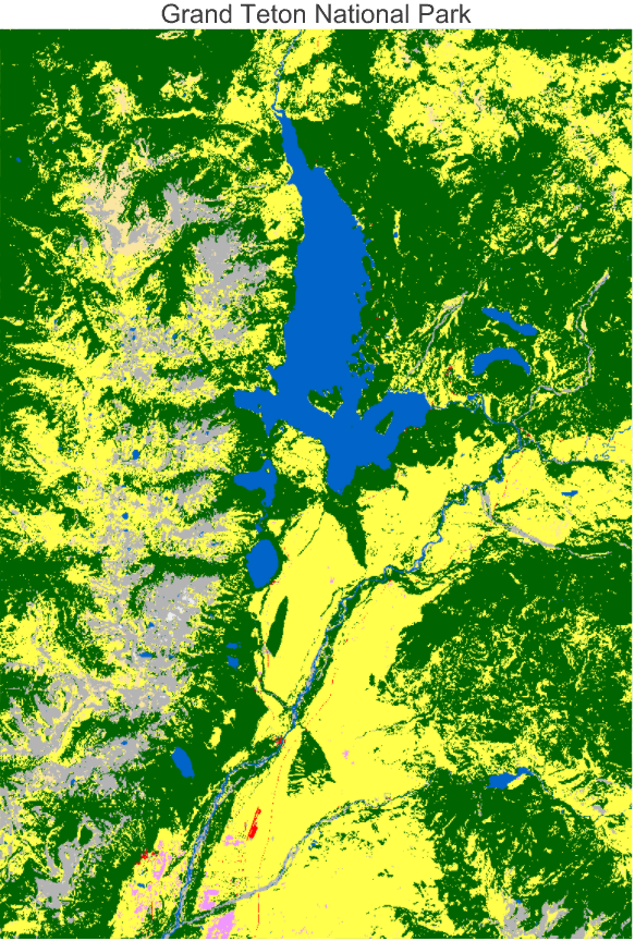
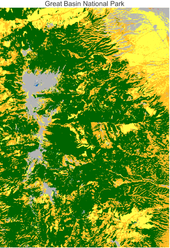
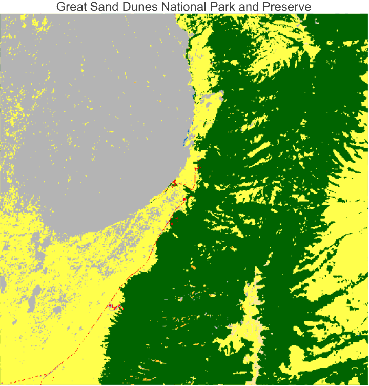
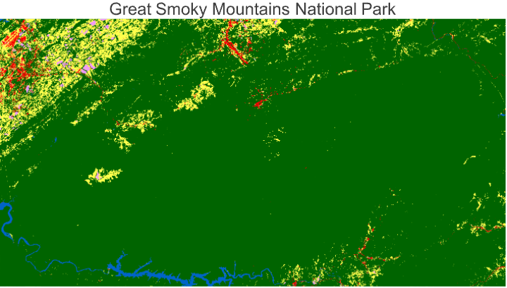
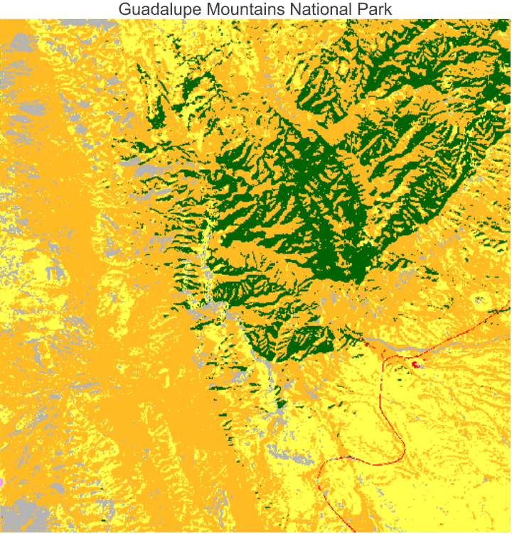
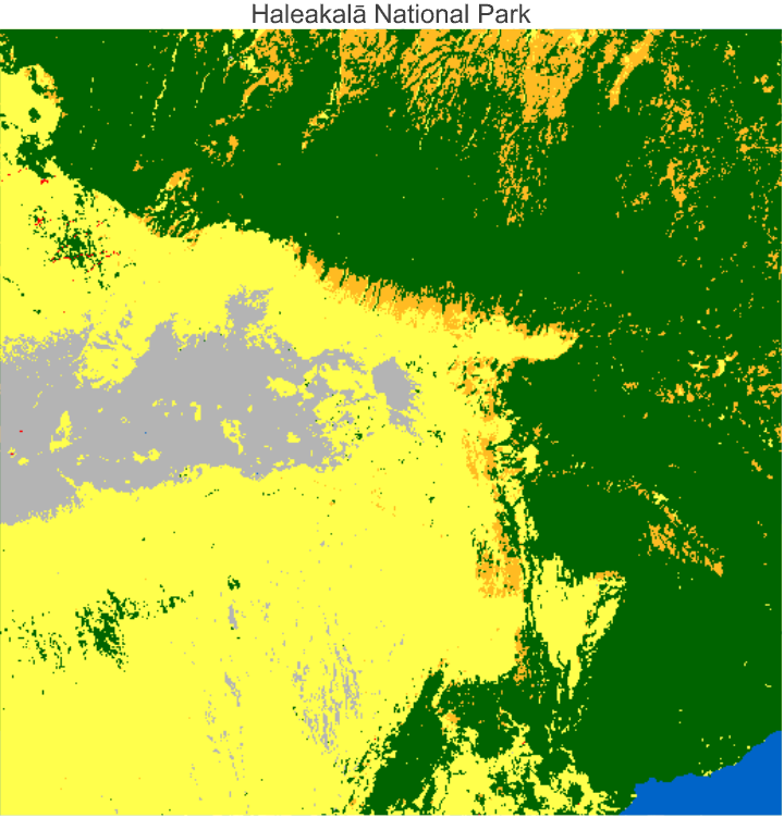
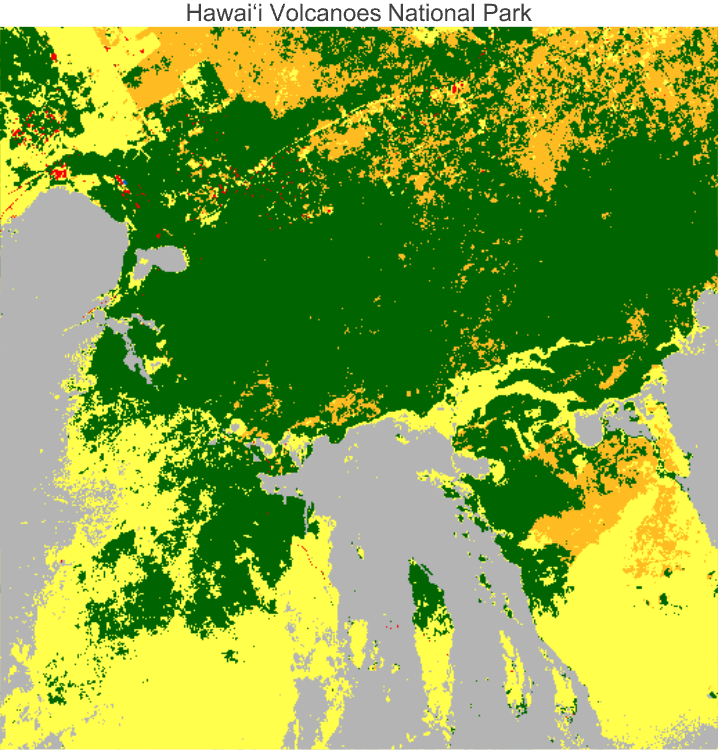
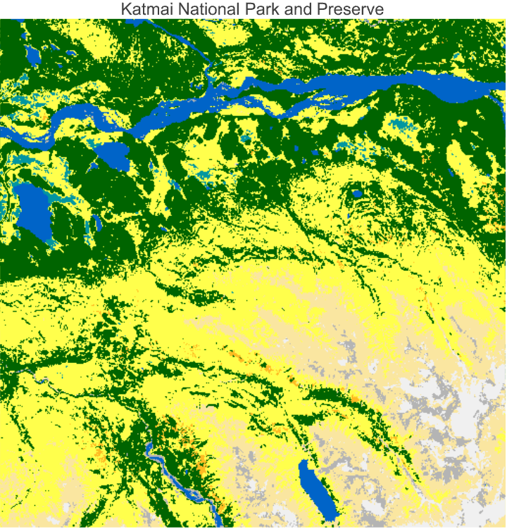
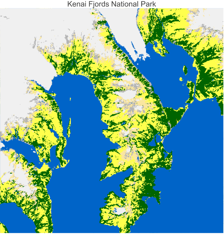
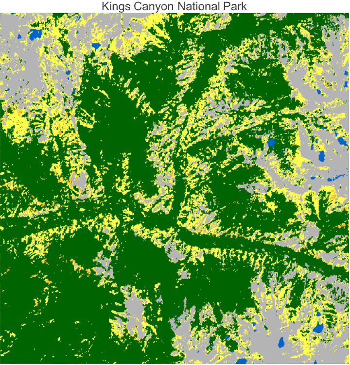
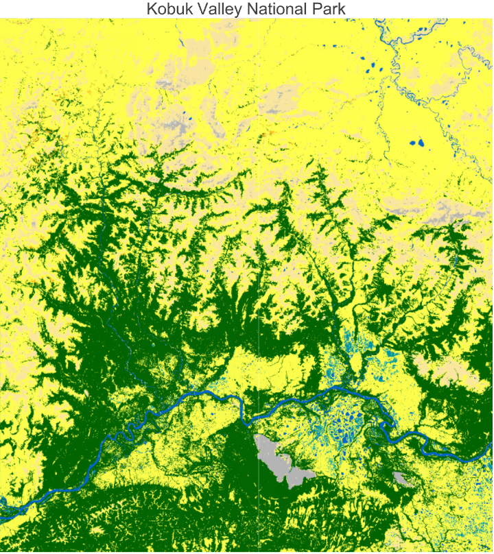
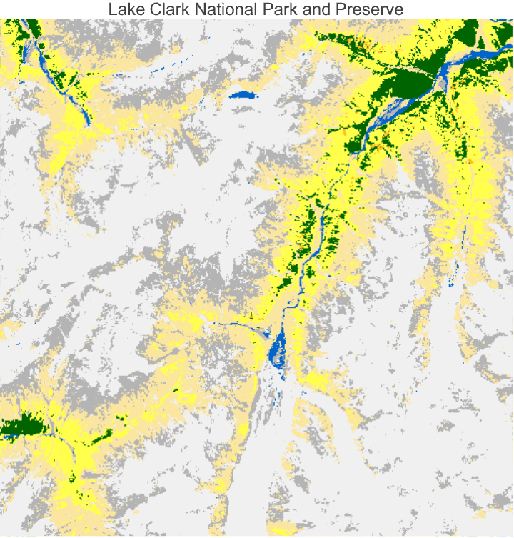
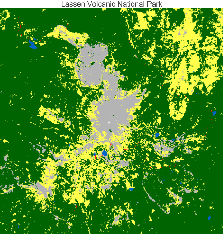
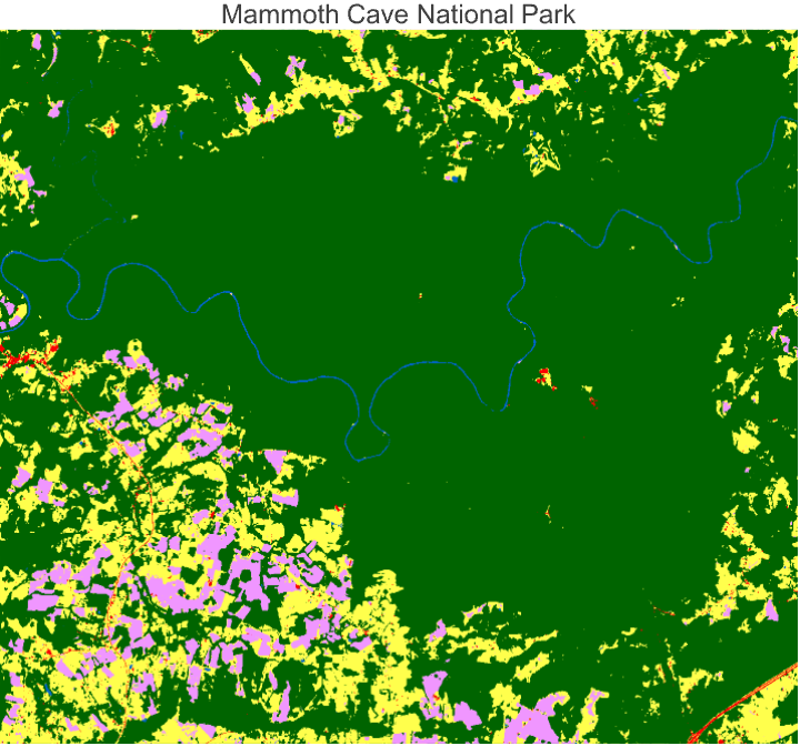
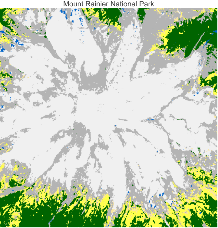
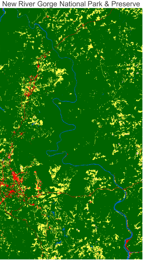
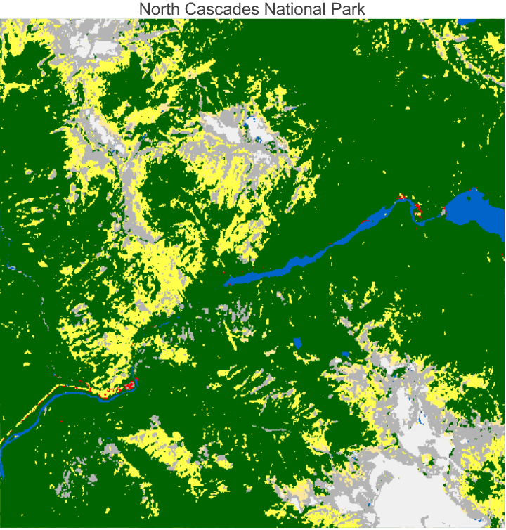
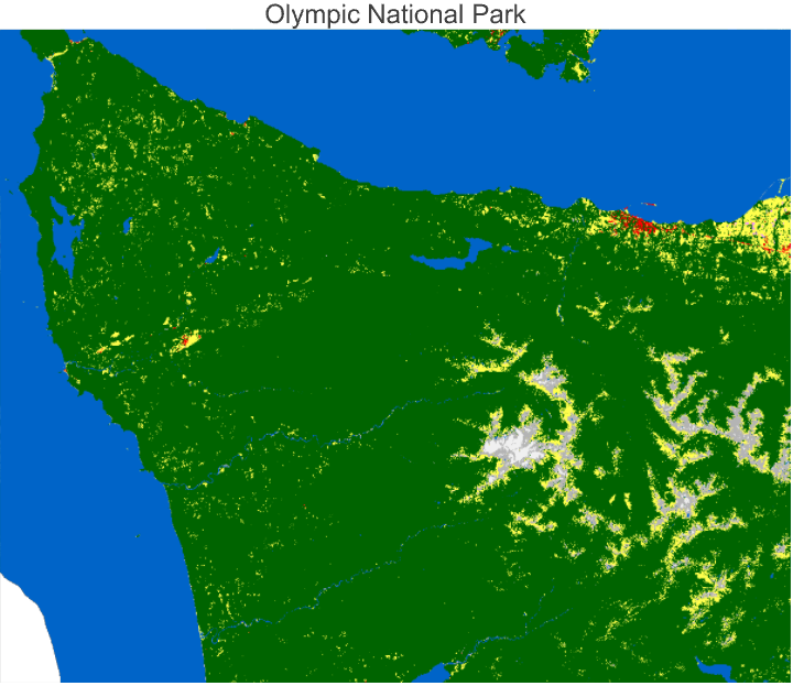
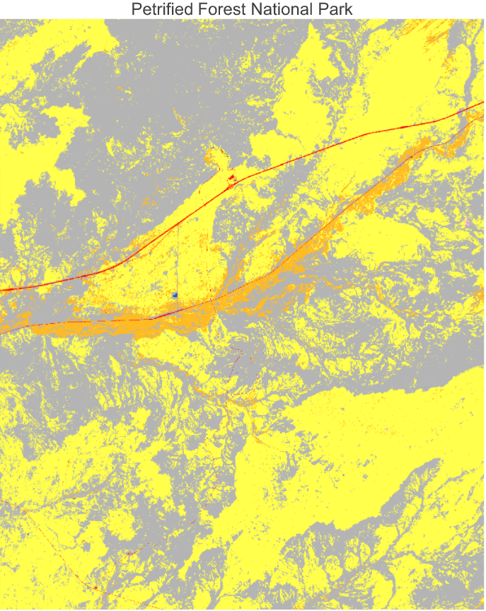
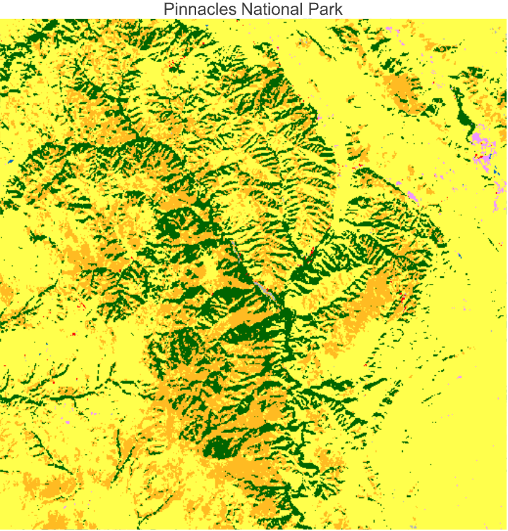
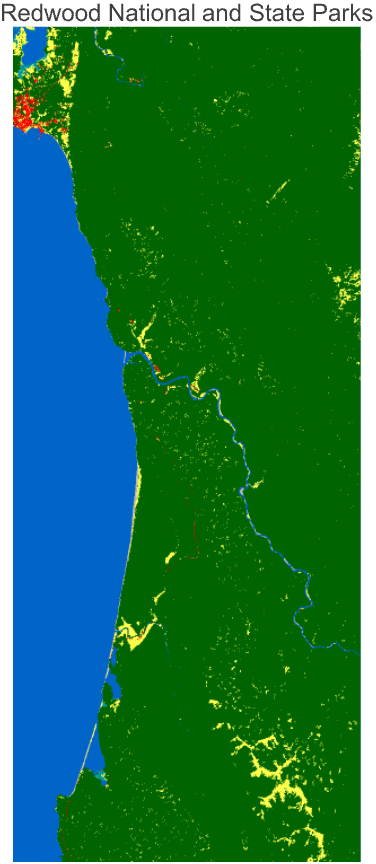
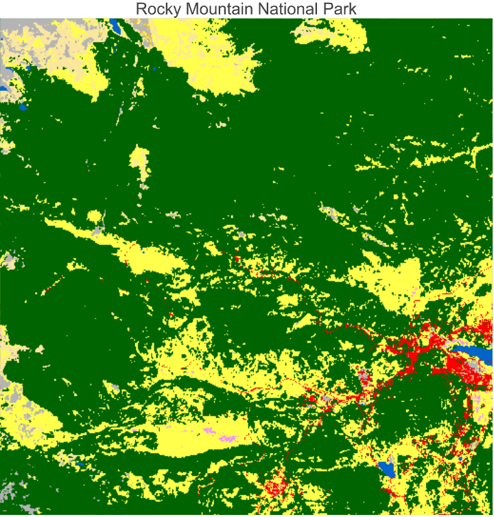
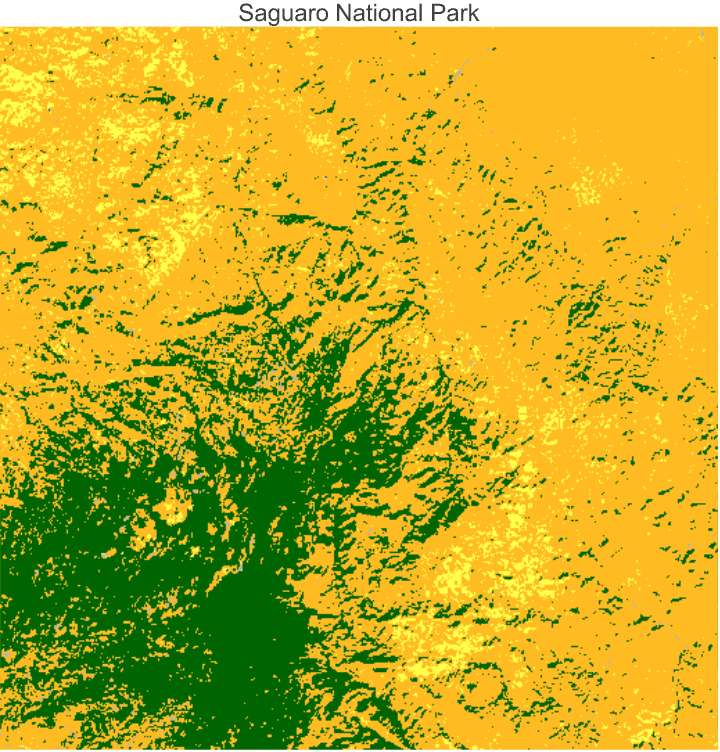
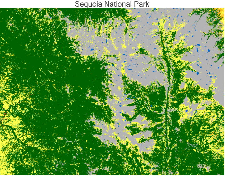
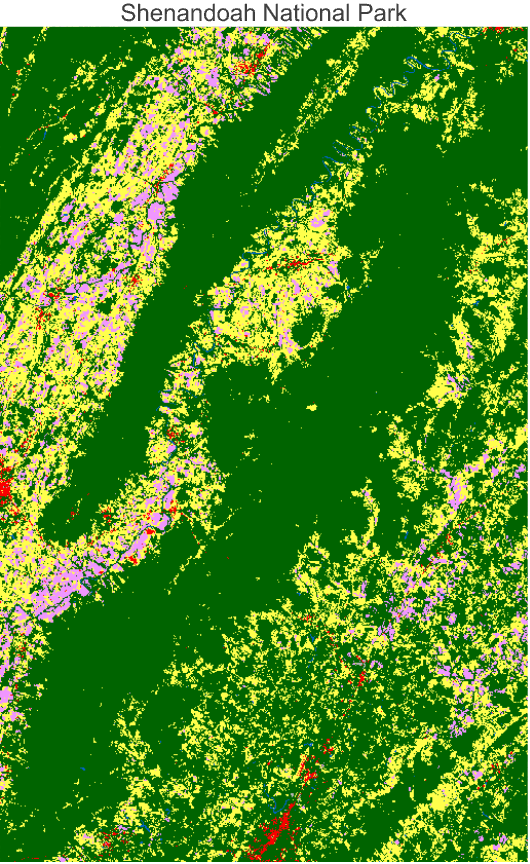
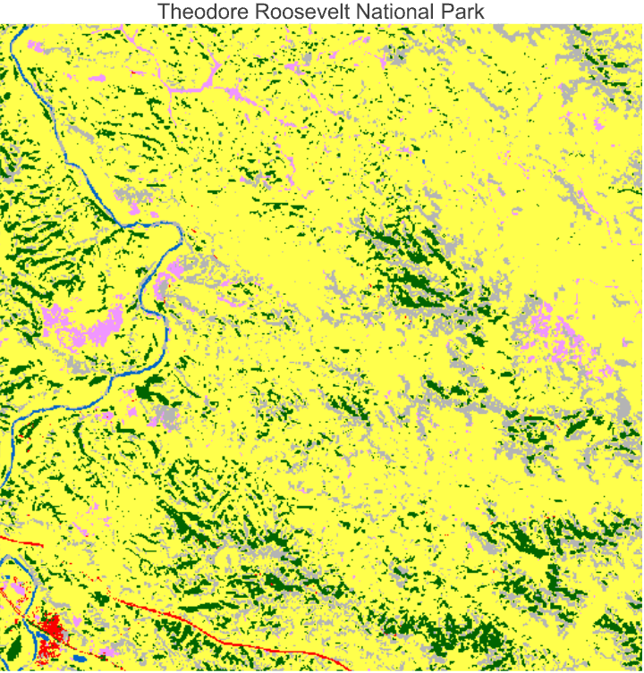
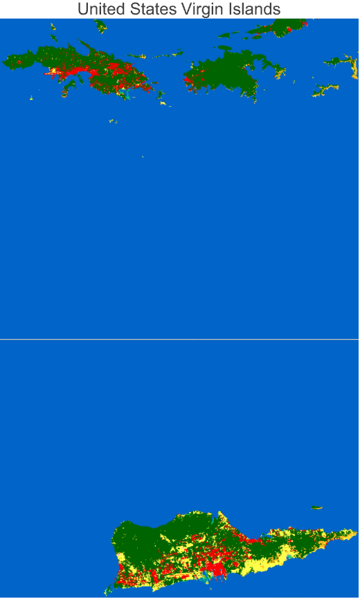
Land cover around US National Parks
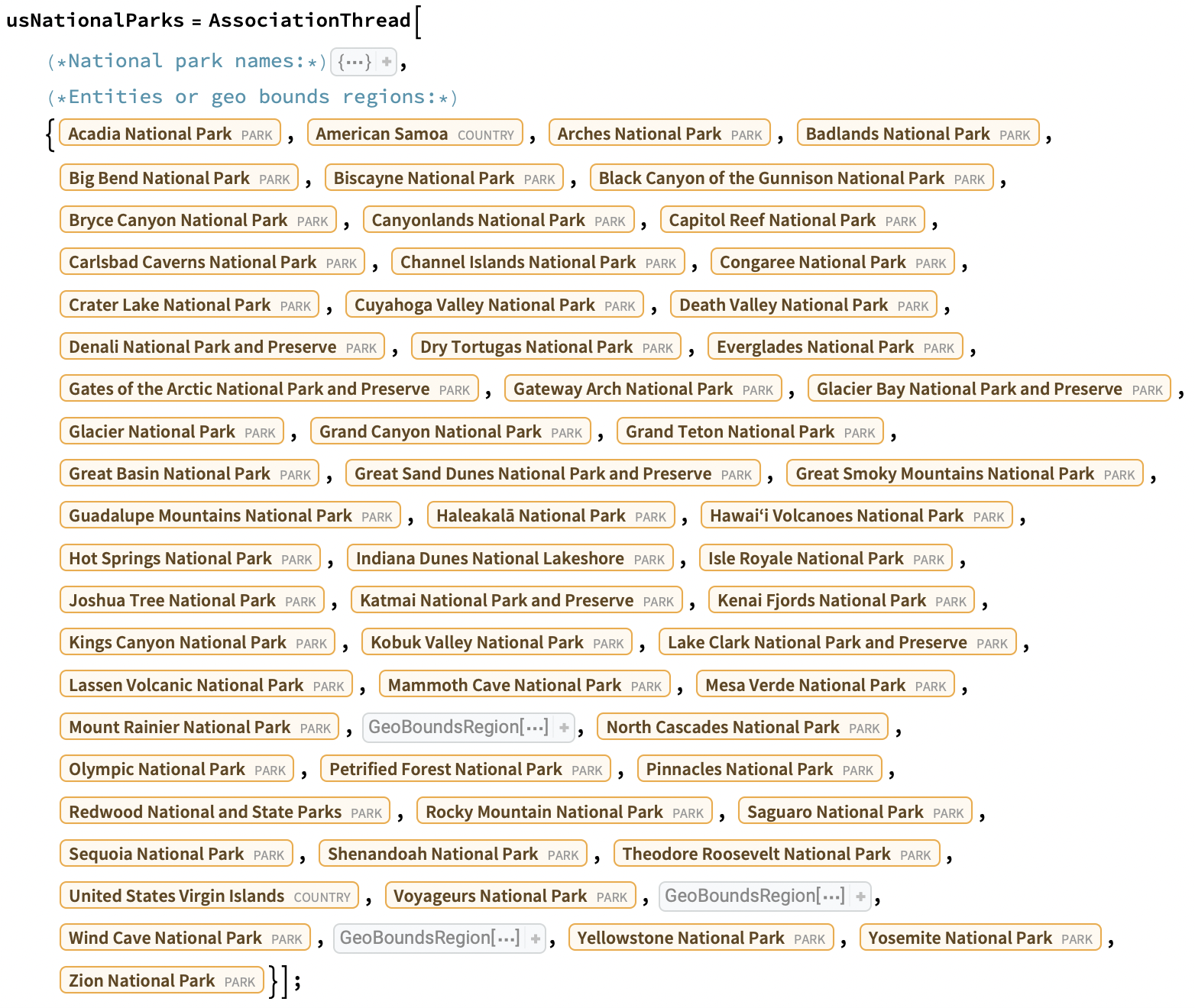
Let's also try this for US national parks. In the last example, we used entities from the Wolfram Knowledgebase to define the geographic footprints of US cities to be plotted. We'll need to to something similar for national but since the knowledgebase does not have built-in entities for every park yet, we'll have to supplement the list with some custom-defined regions as well.
Define an Association representing US national parks:
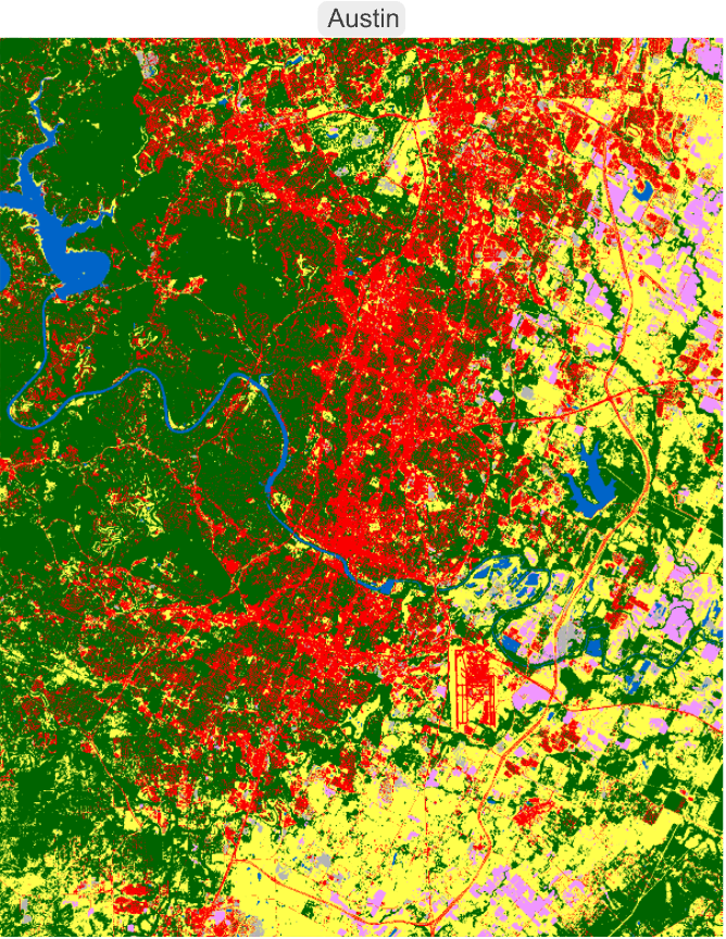
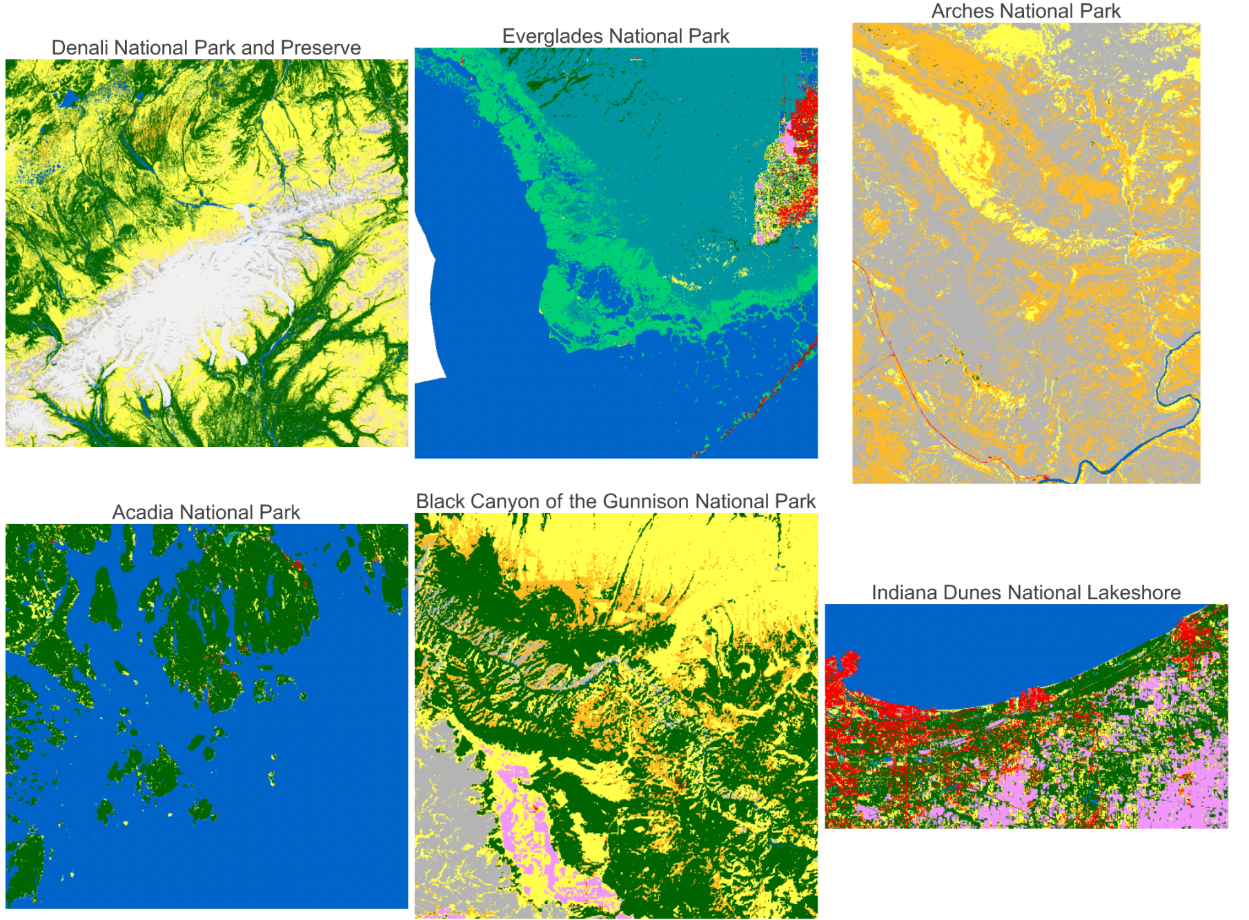
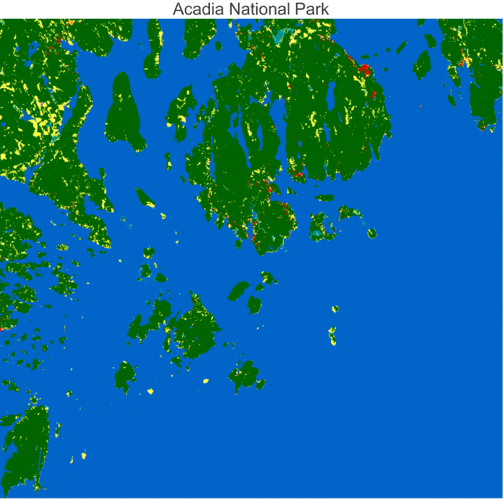
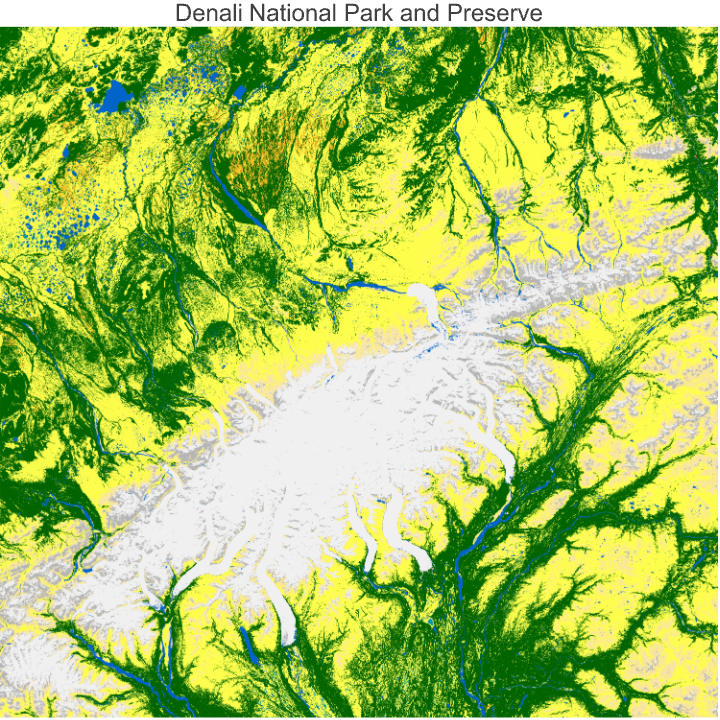
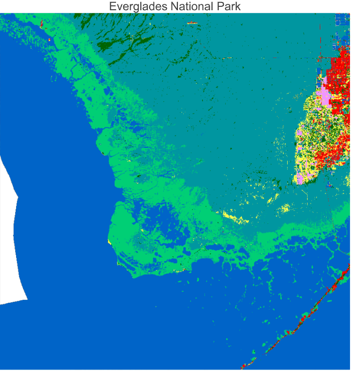
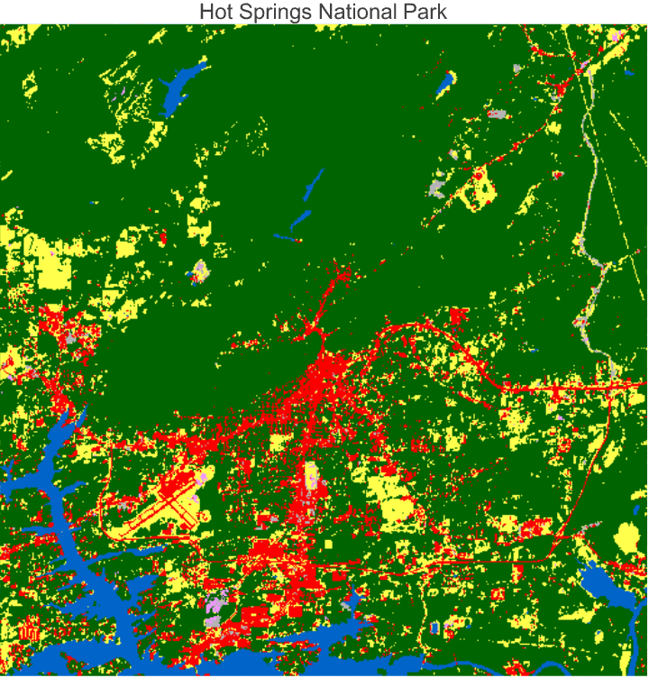
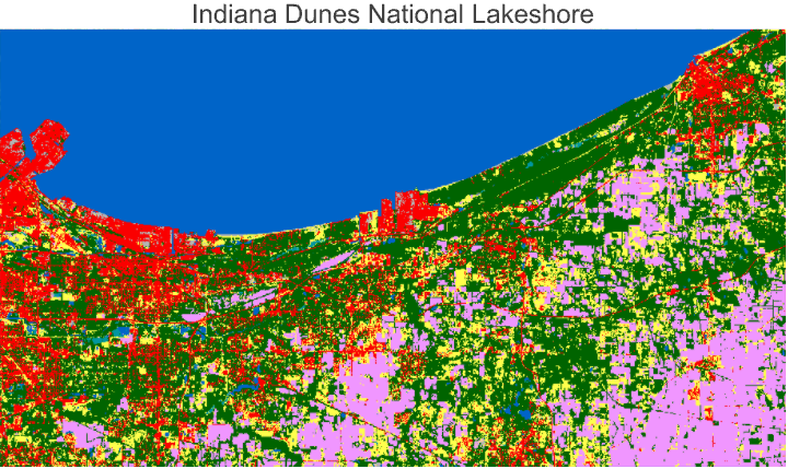
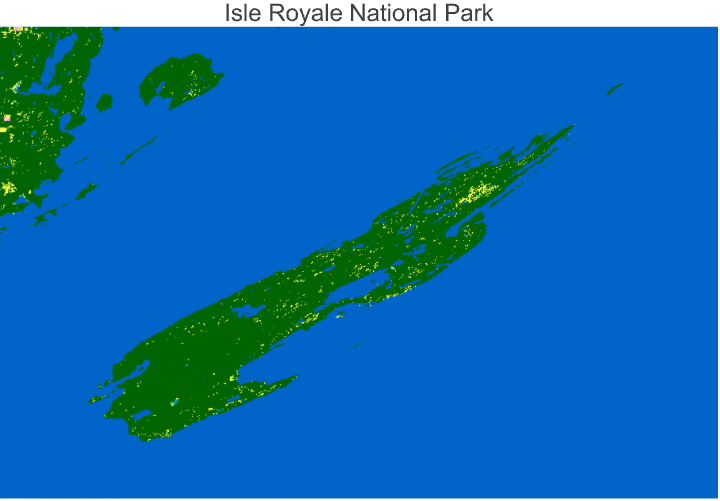
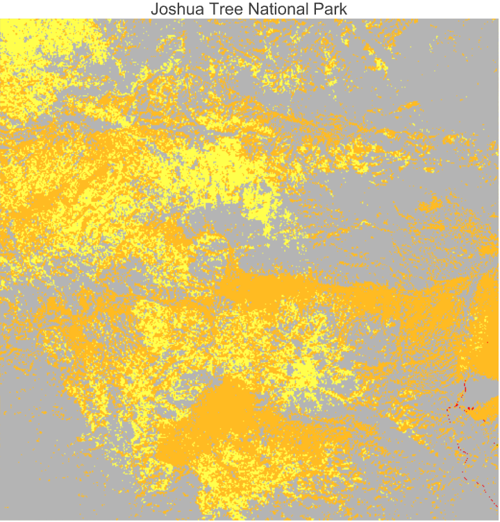
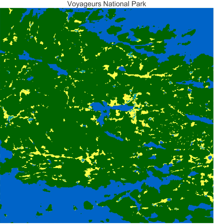
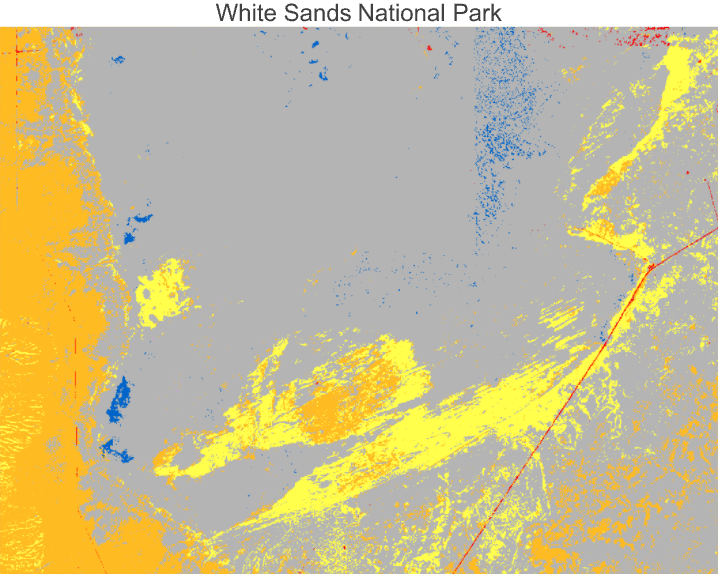
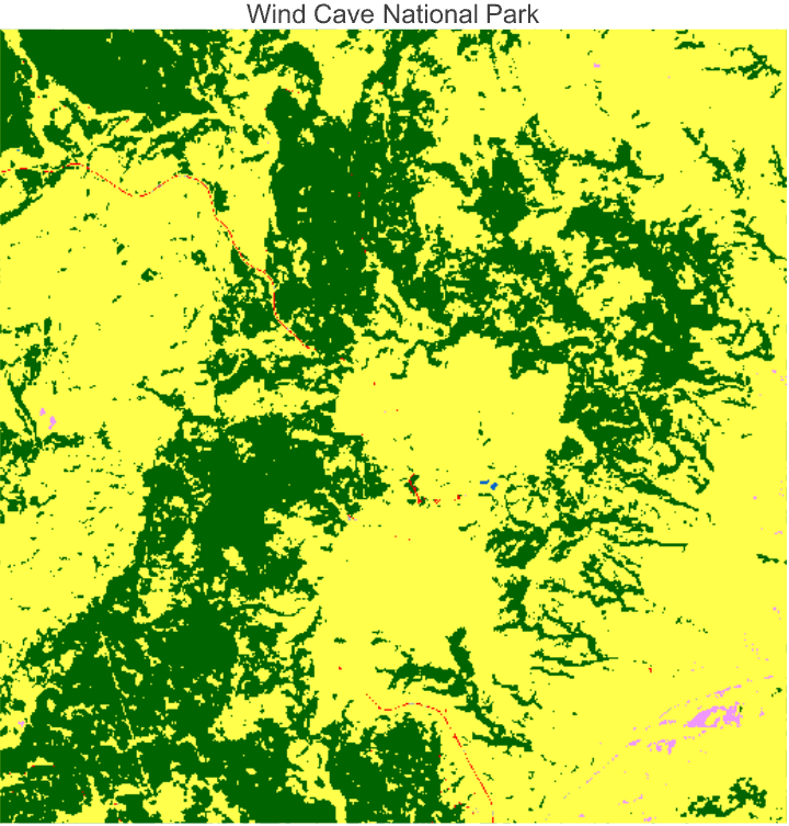
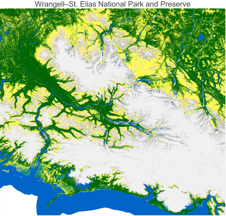
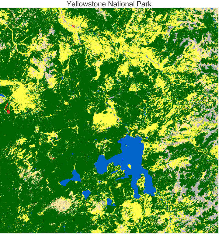
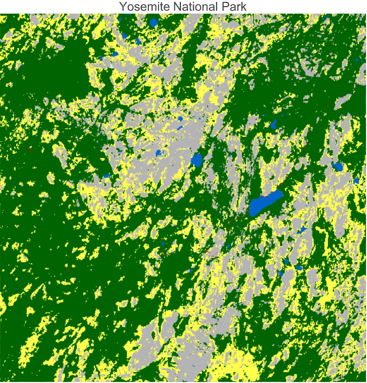
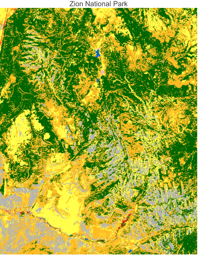
Applying this workflow again to US National Parks, there are important contrasts in the landscape compositions. For instance, Denali and the Everglades have unique dominant cover types: permanent snow and grassland, and herbaceous wetland and mangroves, respectively, that stand apart from the arid shrubland and bare rock of Arches. Other contrasts are defined by topography and hydrography, such as the fragmented coastal forests of Acadia or the steep gradients of the Black Canyon. An outlier, Indiana Dunes is sharply bounded by adjacent urban and agricultural land.
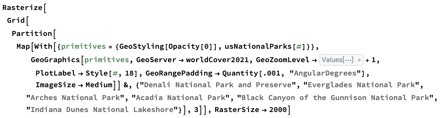
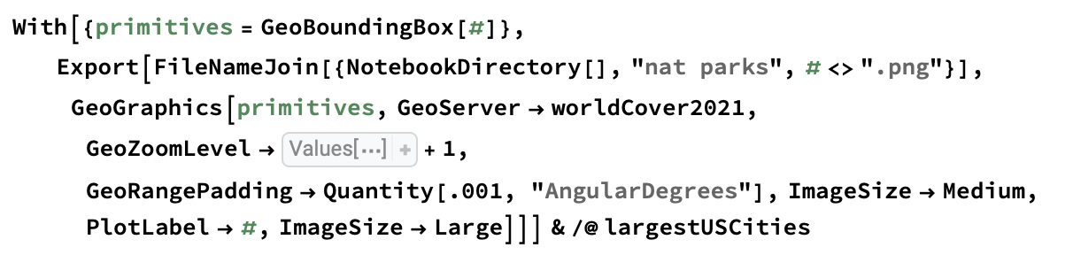
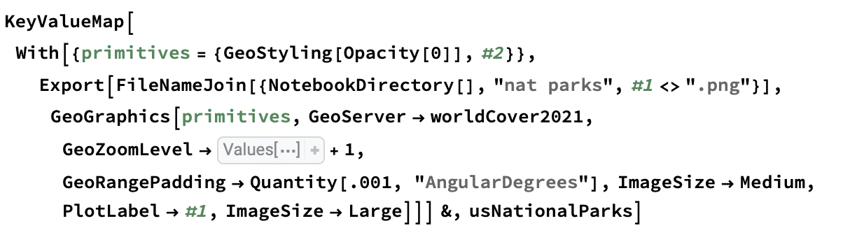
Map the land cover of any US national park:


Connecting to NASA remote sensing services
The ESA WorldCover dataset is a great resource for understanding land cover patterns, and luckily for us, we live in a world in which there are many more. Many remote sensing services are available as map tile servers (WMTS), and two of my favourite providers of high quality free remote sensing imagery datasets of this kind, often with global and sometimes even near real time coverage, are Copernicus Marine and NASA GIBS (Global Imagery Browse Services). You can access NASA GIBS remote sensing imagery using the RemoteSensing paclet, which I've previously written about here.
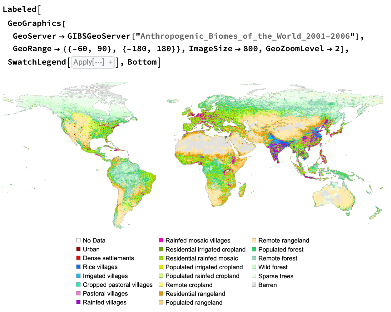
Suppose our reason for consulting ESA LandCover is that we'd like to better understand human environmental impacts globally. In that case, another dataset I'd recommend consulting is the Anthropogenic Biomes (or "Anthromes") map by Ellis & Ramankutty (2008), which classifies Earth's terrestrial surface by the degree and type of human settlements.
The anthropogenic biomes dataset puts human activity at the center of ecological classification, and that makes it an especially compelling tool to study the Anthropocene. It's also conveniently available through NASA GIBS via the RemoteSensing paclet, among over a thousand other remote sensing datasets. Here's how you can install and use this tool yourself:
Run this code to install the paclet:
PacletInstall["PhileasDazeleyGaist`RemoteSensing`"]
Once the paclet is installed, it can be loaded like this:
Needs["PhileasDazeleyGaist`RemoteSensing`"]
Use the RemoteSensing paclet to fetch a map of anthropogenic biomes of the world (Ellis & Ramankutty, 2008):
Sources Cited
WorldCover 2020 v100: Zanaga, D., Van De Kerchove, R., De Keersmaecker, W., Souverijns, N., Brockmann, C., Quast, R., Wevers, J., Grosu, A., Paccini, A., Vergnaud, S., Cartus, O., Santoro, M., Fritz, S., Georgieva, I., Lesiv, M., Carter, S., Herold, M., Li, Linlin, Tsendbazar, N.E., Ramoino, F., Arino, O., 2021. ESA WorldCover 10 m 2020 v100. https://doi.org/10.5281/zenodo.5571936
Ellis, Erle C., and Navin Ramankutty. 2008. Putting People in the Map: Anthropogenic Biomes of the World. https://doi.org/10.1890/070062.