Computational Plant Ecology: Interactive Spatial Network Analysis of a College Garden

August 22, 2025

Note: This post was originally a short technical article I shared on the Wolfram Community forums. For an interactive experience with live demonstrations or to download this text and source code as a Wolfram Notebook, please visit the original post here.

Introduction

About a year ago, a student at College of the Atlantic reached out to me for advice on a capstone project. She was interested in using Wolfram Language to make an interactive map of the college’s Sunken Garden, and exhibiting it as a kind of art installation. To help get her get started, I traced a map of the garden using the image Coordinates tool in a Wolfram Notebook and made two data representations of the garden: a point cloud of plant locations by species and a network of the garden’s paths.

Although her project ended up taking a different direction, the idea stuck with me. After stumbling upon the files recently I was inspired to see if I could build the representations I had made into a fully interactive map. Over the weekend, I dusted off this old notebook and got to work figuring out:

What interesting things can be said about the garden data?
What kind of interactions and interfaces to the data would feel compelling to a general audience interested in the Sunken Garden.
How to package and deploy this experience as a website.

This post is a short reflection on that process, and how I used Wolfram to prototype and design the final website, which you can visit here, or read along to discover bit by bit.

Sketching a digital garden

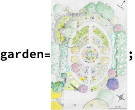
The first step was to import a copy of the map from the brochure:

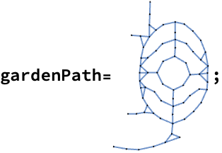
I traced the map image twice: once for plant label coordinates, and once for a rough sample of points along the garden path using the image Coordinates tool described in this tutorial (and I later found this one too). It was a surprisingly meditative experience. I grouped points corresponding to the same species together, and constructed a network representation of the garden path based on my path point sample. I was left with a dataset of plant positions, and a path network.

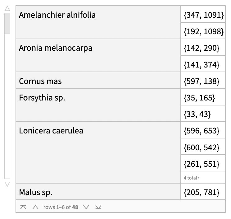
Here’s a preview of the plant positions data:

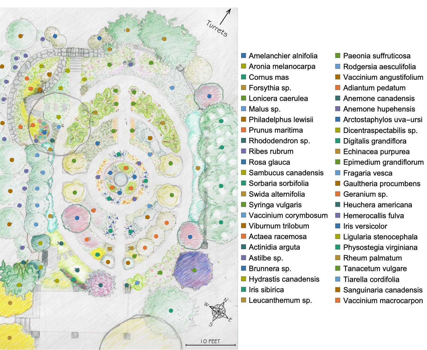
Here’s the original map with digital labels:

In[]:= With[
   {cf = ColorData[91], plantLabels = Normal[plantPositions]}, 
   {colors = cf /@ Range[Length[#]] &@Keys[plantLabels]}, 
   Labeled[HighlightImage[garden, Thread[{colors, Values[plantLabels]}]],SwatchLegend[##, LegendLayout -> {"Column", 2}] & @@ {colors, Keys[plantLabels]}, Right] 
  ]

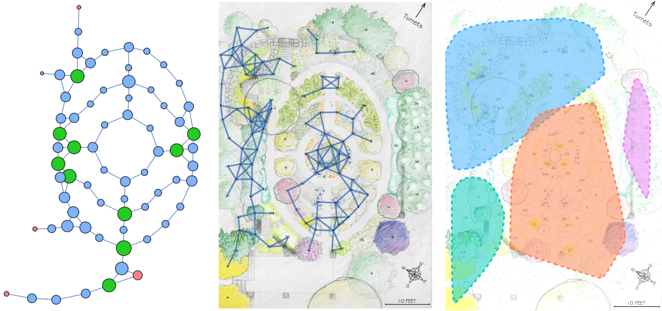
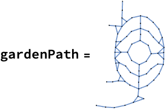
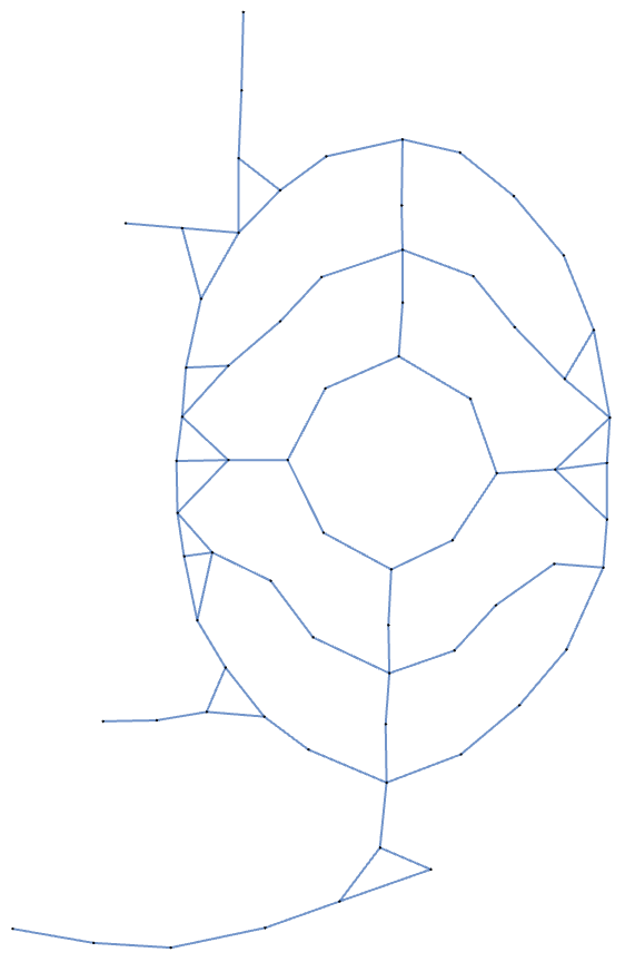
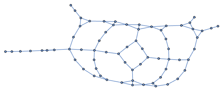
And here’s the network representation of the path:

Investigating the structure of the digital garden

Now that I have these computational representations of the garden, I can use them to answer pretty cool conceptual questions about the data. For example:

On a long random walk through the garden, where am I likely to spend most of my time?
To what extent can I simplify the path network without losing the essence of the path’s design and overall pattern?
What communities do the garden plants form with their neighbors at different scales?

Wandering about the garden

Taking random walks

If I were to walk the garden path randomly or according to some method, I might like to know where I’m most likely to end up after some time. It turns out that this sort of thing is quite easy to simulate assuming that my heuristics for deciding where to go can be well approximated by deterministic or probabilistic rules (and they usually can).

For example, if I walked the path completely at random, I could describe my walk as an algorithm: “Before I take my next step, I’ll choose a random direction along the path.” It turns out that when we aimlessly wander along garden paths, this specific algorithm does not capture what we do well as it results in a high probability of backtracking. In practice, when wandering about a garden, we are much more likely to follow the direction we started with than we are to backtrack. A better algorithmic approximation would be to say that we walk randomly but only allow ourselves to backtrack when we’ve reached a dead end.

Here’s a simulation of such a random walk on the garden path network:

In[]:= ListAnimate[
   With[{n = 100}, Map[
     HighlightGraph[gardenPath, Style[Last[#], StandardGreen], VertexSize -> .5] &, 
     NestList[
      Apply[{#2, RandomChoice[
           With[{possibleNextSteps = VertexOutComponent[gardenPath, #2, {1}]}, 
            If[
             VertexDegree[gardenPath, #2] > 1, 
             Complement[VertexOutComponent[gardenPath, #2, {1}], {#1}],
             possibleNextSteps]]]} &, #] &, 
      {Null, 1}, n]]], 
   AnimationRunning -> False, AnimationTimeIndex -> 5, DefaultDuration -> 10]

Okay, so if I were to randomly wander around the garden for a long time, never backtracking, what locations along the path am I likely to spend most of my time in?

To estimate an answer to this question, we can take a sample of simulated random non-backtracking walks through the garden, and tally the number of visits to each location. We should make the additional assumption that the walks start at one of the garden entrances, chosen at random. Here’s what that looks like with the tallies represented as the sizes of the nodes on the garden path network:

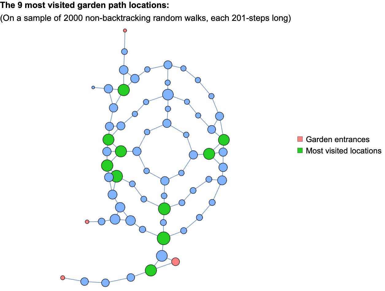
Of course, this is an approximation and the results are biased by the specific choices involved in my translation of the continuous real-world path into a discrete network representation. That said, it’s a reasonable approximation, and one that matches my personal experience of leisurely strolling through the garden with no clear direction.

A short statistical tangent

Across trajectories, the distribution of path-location visit frequencies looks like this:

In[]:= Histogram[
   Flatten[Map[Values@*Normal@*Counts, walks]], 
   ChartStyle -> Lighter[StandardBlue, .5]]

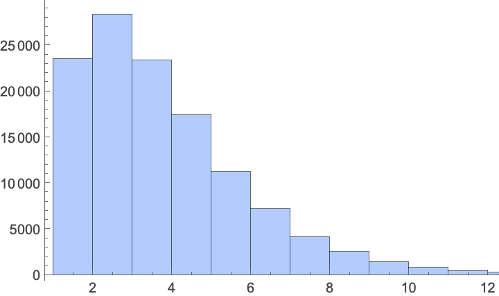
Here’s a model distribution that fits the observed histogram well:

In[]:= dist = FindDistribution[Flatten[Map[Values@*Normal@*Counts, walks]]]

Out[]= MixtureDistribution[{0.798666, 0.201334}, {BenfordDistribution[6], BinomialDistribution[124, 0.0535239]}]

It can be represented as a piecewise function:

In[]:= TraditionalForm[PDF[dist, x]]

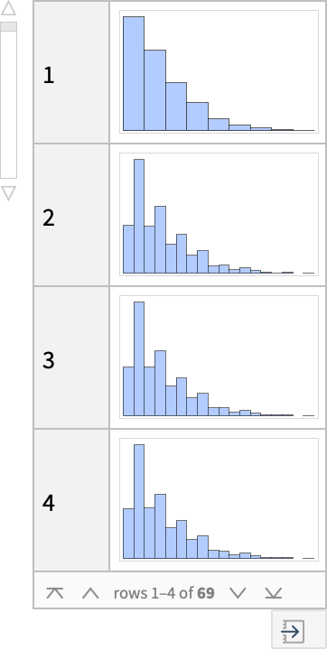
$$\begin{array}{ll} { & \begin{array}{ll} 0. & x>124\lor x<0 \ 0.201334 0.0535239^x 0.946476^{124-x} \binom{124}{x}+0. & 0\leq x<1\lor 6\leq x\leq 124 \ 0.201334 0.0535239^x 0.946476^{124-x} \binom{124}{x}+0.445744 \log \left(\frac{1}{x}+1\right) & \text{True} \ \end{array} \ \end{array}$$

Likewise, I can generate histograms of visit frequencies for specific locations in the garden:

In[]:= Dataset[Dataset[KeySort@DeleteMissing[Normal[Transpose[Dataset[Map[Counts, walks]]]], \[Infinity]]][All, Histogram[#, ChartStyle -> Lighter[StandardBlue, .5]] &], MaxItems -> 4]

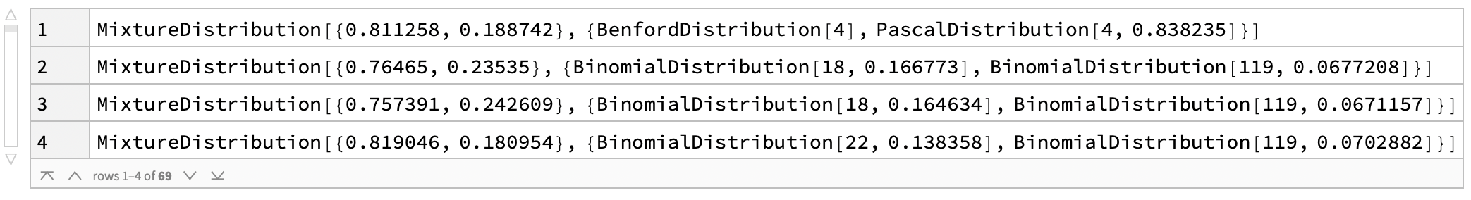
And I can estimate fit distributions to the histograms for each location:

In[]:= Dataset[Dataset[KeySort@DeleteMissing[Normal[Transpose[Dataset[Map[Counts, walks]]]], \[Infinity]]][All, FindDistribution], MaxItems -> 4]

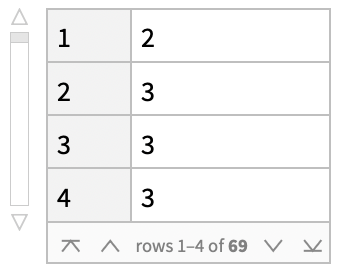
Since these distributions are not normal, we can use the median as our measure of central tendency:

In[]:= Dataset[Dataset[KeySort@Map[Values, GroupBy[Flatten[Map[Normal@*Counts, walks]], First]]][All, Median], MaxItems -> 4]

The skeleton of the garden path

That statistical dive in the last section was helpful for getting a sense of the network’s structure, but it also made me curious about something else: what happens if we start stripping it down to its bones? We have this detailed representation of every path junction and connection, but how much of that complexity is actually doing any work?

How much can I simplify the network without damaging the pattern? This is pretty subjective, as we don’t all agree on what might qualify as a destructive act, or what ought to be preserved in the first place. I’ve chosen to consider distances along the path to be unimportant, but the cycles on the path to be fundamental.

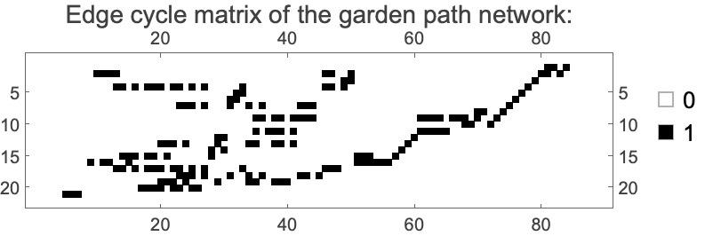
There are 21 cycles in the network. Each cycle is made up of a set of edges on the network, and for every cycle, the edge cycle matrix provides the list of these edges.

In[]:= With[{m = EdgeCycleMatrix[gardenPath]}, 
   ArrayPlot[m, FrameTicks -> True, PlotLegends -> Automatic, ImageSize -> Medium, PlotLabel -> Text[Style["Edge cycle matrix of the garden path network:", 14]]] 
  ]

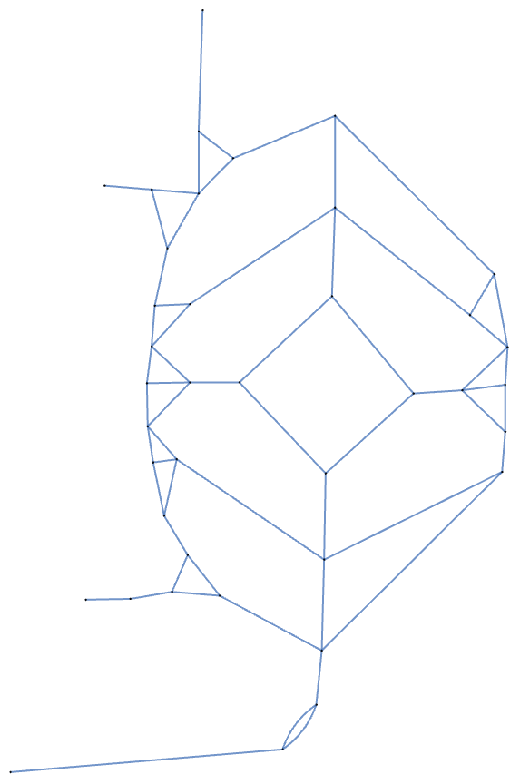
Up to this point I’ve presented the garden path network with its vertices in positions that match their locations on the garden map, but I can use other layouts. Here it is laid out using a spring embedding method:

In[]:= Graph[EdgeList[gardenPath]]

The network looks different, but as far as I’m concerned, it’s the same. The patterns that matter to me (the cycles) are preserved. So how might I simplify the network as much as possible while still preserving all the cycles?

Notice that if distances along the path aren’t important, we can replace any node that has exactly two neighbors with a new edge that goes directly between its neighbors. Essentially, anywhere that we find a connected to exactly two other nodes, we can remove it and directly connect its neighboring nodes. This operation is a form of path pruning that simplifies the network into a kind of ****skeleton representation. The resulting network retains all loop structures but loses path length information.

To apply this simplification to the network, we must be able to perform two tasks: identifying nodes on the network that have exactly two neighbors, and replacing any such node with an edge between its two neighbors. I’ve implemented this functionality below:

In[]:= ClearAll[selectTwoNeighborNodes]
 selectTwoNeighborNodes[g_Graph] := Keys[Select[AssociationThread[VertexList[g] -> VertexDegree[g]], # == 2 &]]

In[]:= ClearAll[deletePassThroughNodes]
 deletePassThroughNodes[g_Graph] := First[NestWhile[{#, First[selectTwoNeighborNodes[#]], Length[selectTwoNeighborNodes[#]]} &@EdgeAdd[VertexDelete[#[[1]], #[[2]]], (UndirectedEdge @@ VertexOutComponent[#[[1]], #[[2]], {1}])] &, {g, First[selectTwoNeighborNodes[g]], Length[selectTwoNeighborNodes[g]]}, TrueQ[Last[#] > 1] &, 1]] /; MemberQ[VertexDegree[g], 2]

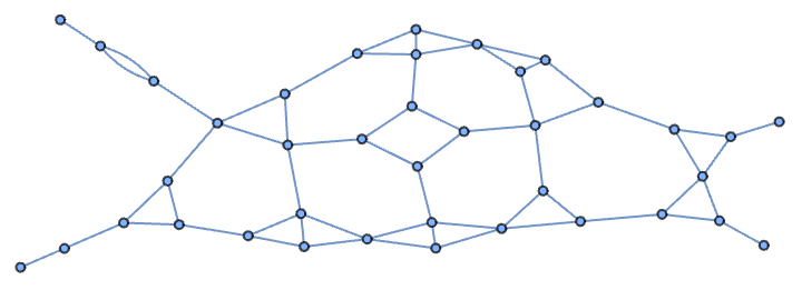
Here’s the simplified path network with a geographic layout:

In[]:= deletePassThroughNodes[gardenPath]

And here it is with a spring layout:

In[]:= Graph[EdgeList[deletePassThroughNodes[gardenPath]]]

Spatial network community analysis of the Sunken Garden plants

Let’s shift from the paths to the plants themselves. Here’s a breakdown of the Sunken Garden’s plant community make-up (the human-designed component):

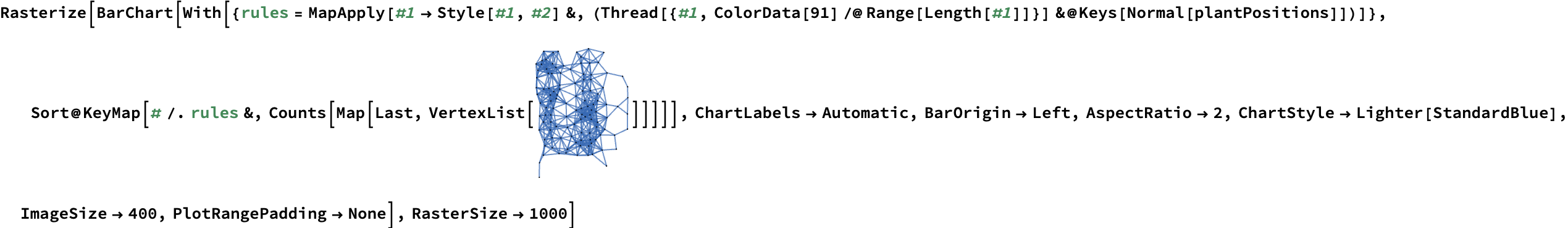
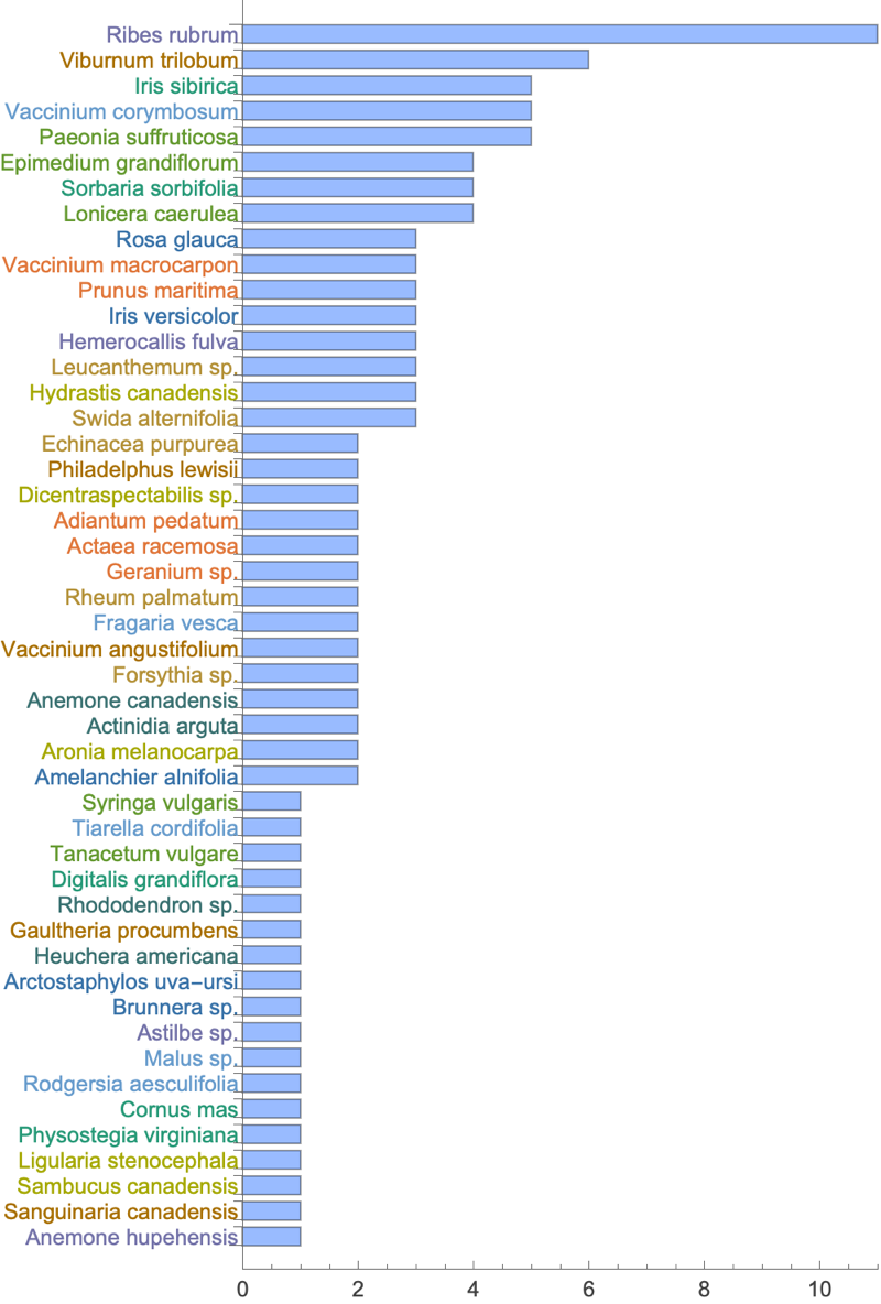
We’ve been thinking about how people might move through the space, but the plants have spatial relationships of their own: clusters and neighborhoods that form based on proximity, growing conditions, etc. Can we detect these plant communities computationally? How do they change depending on the scale at which we search for them?

To answer these questions, we need to know how strongly plants interact with each other as a function of their distances from one another. This will vary from plant to plant and between plant pairs as individual plants may prefer to interact with some species above others. Since we don’t have this information readily available but still have the intuition that the degree of interaction between plants is somewhat a function of the distance between them, I’m going to make an obviously wrong assumption that will still turn out to be instructive: That the amount of interaction between any two plants decreases linearly as a function of mutual distance, and that the slope and y intercept are the same across plants.

Botanists, suspend your disbelief! But you’re right to ask: why should we decide to make this assumption, especially if we expect it to be inaccurate? The answer is that although it flattens the world and its complexity somewhat, it’s about to allow us to tease out some other interesting properties of the network of plants in the garden.

Let’s imagine that our assumption is true: That the amount of interaction that happens between any two plants is described by the same linear function of the distance between the plants. In that case, to model the network of interactions between plants at a spatial scale $r$, we can simply imagine disks of radius $r$ centered at every plant and take note of which nodes fall inside what disks. Wherever a plant finds itself in a disk, we assess that the plant is close enough to its neighbor at the center of the disk for them to interact in some way. When two plants interact at a designated scale, we draw a link between them, building a model spatial network of the Sunken Garden’s plant interactions.

Here’s an interactive demonstration of the process:

In[]:= Manipulate[
   Show[
    garden, 
    With[
     {g = NearestNeighborGraph[#, {All, N[172/10]*radius}] &@Flatten[Values[Normal[plantPositions]], 1]}, 
     With[
      {labelRules = ((Thread[Keys[#1] -> Callout @@@ #1] &)[Flatten[Thread /@ Reverse /@ Normal[Normal[plantPositions]]]])},
      {edges = EdgeList[g] /. labelRules}, 
      Graph[Values[labelRules], edges, VertexCoordinates -> Thread[Values[Association[labelRules]] -> GraphEmbedding[g]], EdgeStyle -> Thick] 
     ] 
    ]], {{radius, 5}, 0, 10}, SaveDefinitions -> True]

Since we can now estimate spatial networks of plant interactions based on distance, we can also apply community detection methods to these networks to make estimates of where interactions concentrate in the network at different scales:

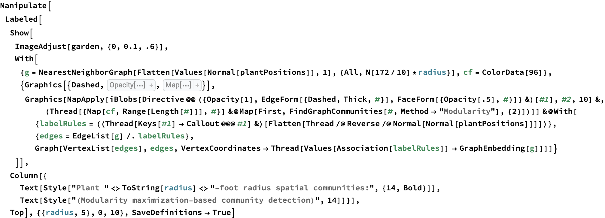
This spatial network analysis reveals how the Sunken Garden’s plant communities might emerge at different interaction scales. For radii under approximately 1.75 feet, there are no detected communities, as no plants are within that distance of one another. At radii between two and three feet, we see tightly clustered micro-communities. For radii between four and five feet, we find medium-sized communities that overlap meaningfully with the intentional design and pattern of the garden. At this scale, the garden path seems to contribute to delineating the community structure. As we increase the interaction radius to six to ten feet, these smaller communities merge. For a radius of ten feet, there are four detected communities, two of which cover the majority of the garden:

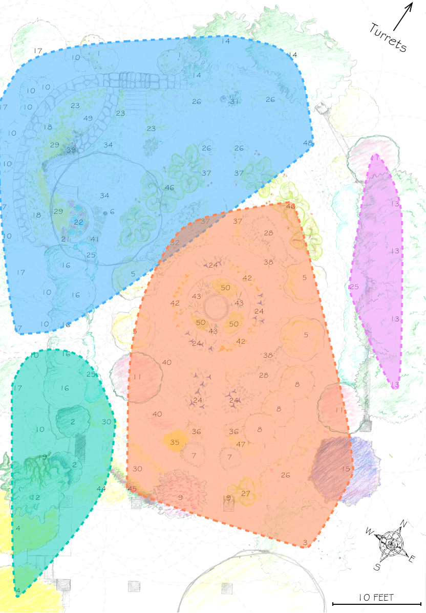
The modularity-based community detection shows that even under our simplified assumption of uniform distance-based interactions, the garden shows clear spatial clustering that changes meaningfully with scale. At intermediate scales, the communities appear to align with the garden’s major design elements—the central beds, perimeter plantings, and transitional zones.

Of course, our linear distance model is a deliberate oversimplification. In reality, plant interactions depend on species compatibility, root systems, light requirements, soil preferences, and many other factors that vary between species pairs. Some plants are natural companions that thrive in close proximity, while others compete aggressively or have allelopathic effects on their neighbors.

Despite these limitations, the spatial community analysis shows how computational methods can reveal organizational patterns in designed landscapes that might not be immediately apparent. The scale-dependent nature of the detected communities suggests that the Sunken Garden operates as a multi-layered spatial system. The alignment of intermediate-scale communities with major design elements reflects the fact that the garden’s layout creates natural zones of interaction.

Plant data analysis

I reached out to some contacts at the college for information about the garden plants that I could add to the garden website. [Name], the current Sunken Garden curator shared a species information booklet he wrote with me, the Edible Plant List of the Sunken Garden, which contained all sorts of helpful information about the plants. I used OCR alongside a mix of methods to extract the data from the booklet, and convert them to a JSON dataset, which I’ve reproduced here:

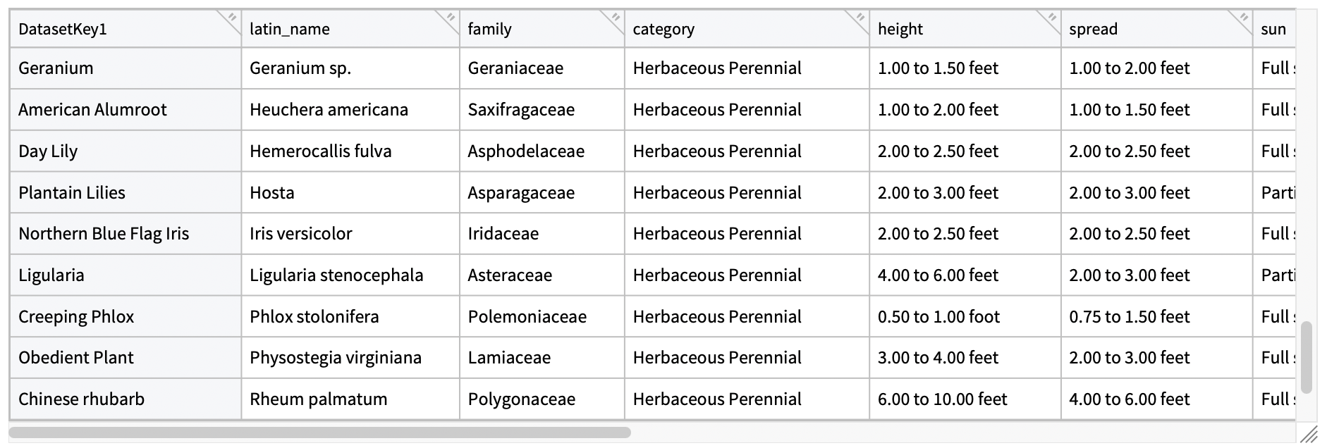
The dataset contains detailed information about 56 plant species in the Sunken Garden, including their Latin names, families, growing requirements, physical characteristics, and seasonal information.

The data reveal clear patterns in plant selection. Most species are adaptable to varying light conditions:

In[]:= Dataset[ReverseSort@KeyMap[First, Normal[Counts[Values[Dataset[ConstructColumns[plantData, "sun"]]]]]]]

Full sun to partial shade	Partial shade to full shade	Full sun	Partial shade
32	13	8	3

The tally of plant water requirements show a similar preference for adaptable species:

In[]:= Dataset[ReverseSort@KeyMap[First, Normal[Counts[Values[Dataset[ConstructColumns[plantData, "water"]]]]]]]

Medium	Medium to wet	Dry to medium	Low
38	11	6	1

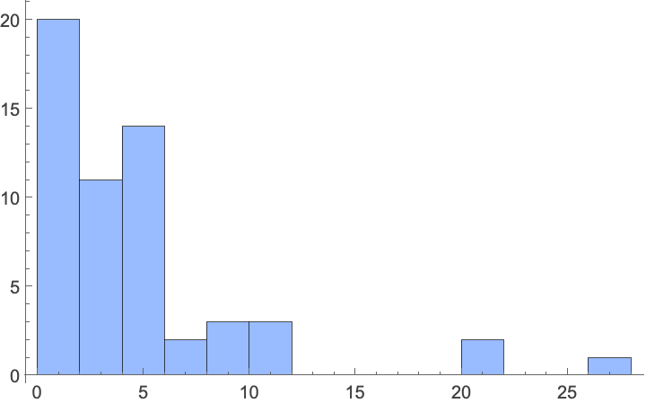
Plant heights cluster around smaller values, with almost all species under 10 feet, and most 5 feet or under:

In[]:= Histogram[Flatten[Normal[Values[Dataset[ConstructColumns[plantData, {
         "height" -> Function[Around[Mean[#], Mean[#] - Last[#]] &@ToExpression[
             "{" <> StringReplace[#"height", {" to " -> ",", " feet" | "foot" -> ""}] <> "}"]]}]]]]], 
   PlotRange -> Full, ChartStyle -> Lighter[StandardBlue]]

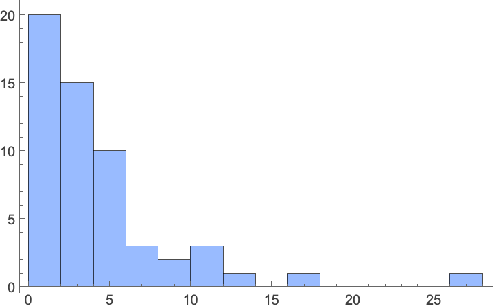
Spread values show a similar pattern, with most plants staying compact:

In[]:= Histogram[Flatten[Normal[Values[Dataset[ConstructColumns[plantData, {
         "spread" -> Function[Around[Mean[#], Mean[#] - Last[#]] &@ToExpression[
             "{" <> StringReplace[#"spread", {" to " -> ",", " feet" | "foot" -> ""}] <> "}"]]}]]]]], 
   PlotRange -> Full, ChartStyle -> Lighter[StandardBlue]]

Height and spread scatter plot with a LOESS fit:

In[]:= ListFitPlot[Normal[Values[Dataset[ConstructColumns[plantData, {
        "height" -> Function[Around[Mean[#], Mean[#] - Last[#]] &@ToExpression[
            "{" <> StringReplace[#"height", {" to " -> ",", " feet" | "foot" -> ""}] <> "}"]], 
        "spread" -> Function[Around[Mean[#], Mean[#] - Last[#]] &@ToExpression[
            "{" <> StringReplace[#"spread", {" to " -> ",", " feet" | "foot" -> ""}] <> "}"]]}]]]], 
   PlotRange -> Full, PlotFit -> "Local", PlotFitElements -> "BandCurves"]

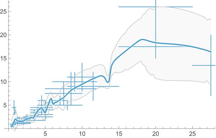
The plant data analysis confirms that the Sunken Garden prioritizes adaptable, compact species that do well in variable conditions.

Packaging and deploying a website

The primary goal was always to create an accessible digital companion for garden visitors. The website allows people to click on plant locations for detailed species information, click on path nodes to see what plants are within short and medium distance radii of that spot, and toggle between different organizational views (by species, growing requirements, bloom time, and other characteristics).

The computational analyses presented here emerged from my curiosity about the underlying spatial patterns in this designed landscape. While some insights, like meaningful plant interaction distances, influenced minor interface details, the mathematical investigations are primarily an addendum for visitors interested in exploring the garden through a computational lens.

Here’s the sunken garden website directory tree:

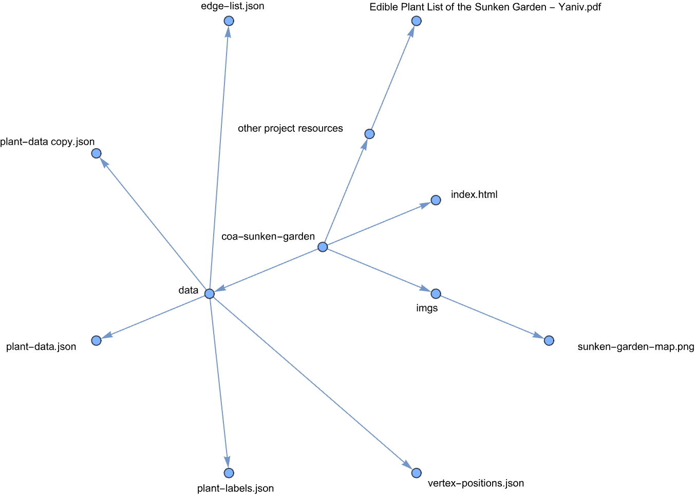
The website uses a straightforward structure with JSON data files containing the computational representations developed through the Wolfram analysis. The network visualizations use the force-graph library, while most of the implementation work went into defining the logic for different information modals and user interactions. I deployed the site using GitHub Pages for free hosting.

Parting thoughts

Gardens occupy a middle ground between artificial and natural systems. They blend human intention with processes that operate beyond conscious control. This hybrid status makes them revealing subjects for computational analysis because they illuminate how spatial patterns emerge independent of design intentions.

When the distance-based community detection occasionally aligns with garden design elements, it raises interesting questions about the relationship between our analytical frameworks and spatial reality. The patterns emerge from specific modeling choices - the distance thresholds we select, the assumption that all plants interact uniformly, the particular community detection algorithm we apply. Yet the occasional alignment with actual design elements suggests these simplified models can still capture meaningful aspects of spatial organization.

The computational approach offers a way to think systematically about spatial relationships, even when our assumptions are deliberately oversimplified. Gardens provide a useful testing ground for these methods precisely because we can compare analytical results against known design intentions and see where the models succeed or fall short.

You can explore the interactive map here.

Appendix: Code Initializations

Project variables

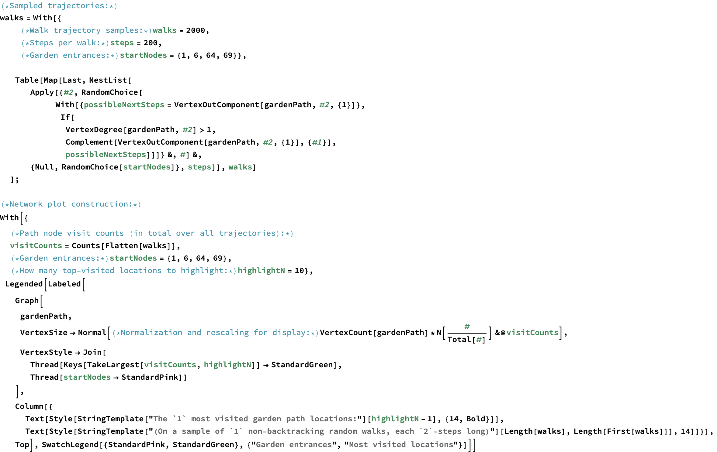
In[]:= walks = With[{
         (*Walk trajectory samples:*) walks = 2000, 
         (*Steps per walk:*) steps = 200, 
         (*Garden entrances:*) startNodes = {1, 6, 64, 69}}, 
        
        Table[Map[Last, NestList[
           Apply[{#2, RandomChoice[
                With[{possibleNextSteps = VertexOutComponent[gardenPath, #2, {1}]}, 
                 If[
                  VertexDegree[gardenPath, #2] > 1, 
                  Complement[VertexOutComponent[gardenPath, #2, {1}], {#1}],
                  possibleNextSteps]]]} &, #] &, 
           {Null, RandomChoice[startNodes]}, steps]], walks] 
        ];

In[]:= dist = FindDistribution[Flatten[Map[Values@*Normal@*Counts, walks]]];

In[]:= ClearAll[selectTwoNeighborNodes]
 selectTwoNeighborNodes[g_Graph] := Keys[Select[AssociationThread[VertexList[g] -> VertexDegree[g]], # == 2 &]]

In[]:= ClearAll[deletePassThroughNodes]
 deletePassThroughNodes[g_Graph] := First[NestWhile[
         {#, First[selectTwoNeighborNodes[#]], Length[selectTwoNeighborNodes[#]]} &@EdgeAdd[VertexDelete[#[[1]], #[[2]]], (UndirectedEdge @@ VertexOutComponent[#[[1]], #[[2]], {1}])] &, 
         {g, First[selectTwoNeighborNodes[g]], Length[selectTwoNeighborNodes[g]]}, TrueQ[Last[#] > 1] &, 1]] /; MemberQ[VertexDegree[g], 2]

Misc tools

Drawing blobs

Define a function to draw blobs:

In[]:= ClearAll[iBlobs]
 iBlobs[style_, pts_, size_] := Block[{epts}, 
       epts = Flatten[Tuples[CoordinateBounds[#, size]] & /@ pts, 1]; 
       {style, FilledCurve@BSplineCurve[
              MeshPrimitives[ConvexHullMesh[epts], 1][[All, 1, 1]], 
              SplineClosed -> True, SplineDegree -> 2]}]